The task of calculating the flux of carbon dioxide (CO₂) between the atmosphere and the ocean has often been considered as two separate problems: to measure or predict the difference in CO₂ concentration across the air-sea interface, which is the thermodynamic driving force for the flux, and to investigate the rate of exchange by which this must be multiplied, which is the kinetic parameter often known as the "transfer velocity". This transfer velocity is a function primarily of windspeed and temperature, but is also influenced by many other minor processes. One of these processes, the enhancement of the exchange rate of CO₂ due to its chemical reaction with water and the possibility that this may be catalysed by an enzyme produced by marine microalgae (phytoplankton), is the focus of most of this thesis.

However, before introducing the various factors which control the transfer velocity, and particularly the chemical enhancement effect, later in this chapter, and introducing the catalysis by enzyme produced by marine algae in chapter two, I will begin with an brief overview of the global carbon cycle and its role in controlling the climate, the reason behind the intense research effort which has been directed at this topic for the last 40 years. I will also consider briefly the various different approaches which have been used to measure or predict the global air-sea CO₂ flux, and mention the physical and biological processes which control the thermodynamic parameter, the partial pressure of CO₂ in the surface ocean. It is the complex combination of such processes which dictates the need for indirect approaches to measuring the CO₂ transfer velocity. Moreover it will be seen later that, when we consider chemical enhancement and various other minor processes affecting the transfer velocity, the kinetic and thermodynamic parameters of air-sea CO₂ exchange are not independent, and so it is essential to consider the effect of intercorrelation between processes in order to make a reasonable estimate of the finely balanced net global air-sea CO₂ flux.

Thus the structure of this introductory chapter is to start with the global scale problem, and from there to gradually zoom in to focus on the small-scale processes of CO₂ transfer across the sea-surface microlayer (see Section 1.2.1 ). The reader should bear in mind that much of the science of this topic has of course evolved in the opposite direction, beginning with research into small-scale processes and measurement techniques, whose results were later incorporated into the global models and calculations. The history of research into the global carbon cycle has recently been reviewed by Heimann (1997).

Moreover, this brief introduction to the ocean carbon cycle and air-sea CO₂ flux can only skim the surface of a vast topic. For example, there are now many hundreds of papers reporting surface water pCO₂ measurements from research cruises in various regions of the ocean in different seasons, which also discuss the various factors which might explain the measured data, and the local fluxes calculated using various transfer velocity parameterisations. So many results could not be summarised in this thesis, so here only a few references will be given to highlight particular issues. Similarly, there can only be room below for a handful of references regarding the vast topic of global climate change.

1.1.1 CO₂ and global climate.

Molecules of greenhouse gases such as CO₂ can raise their rotational or vibrational energy levels by absorbing infra-red photons emitted from the surface of the earth in response to solar heating. These molecules then reemit infra-red photons in all directions, some of them back towards the earth's surface, which must therefore adjust to a warmer temperature in order to restore the heat balance between incoming and outgoing radiation. The first prediction of the magnitude of this "greenhouse effect" was made by Arrhenius (1896), and has since been found to be remarkably accurate since it included the effect of water vapour amplifying the warming due to CO₂ (more on this below).

Converting carbon and oxygen to CO₂ releases energy, and so the coexistence of a high concentration of O₂ in the atmosphere, in contact with large stores of organic and inorganic carbon in the biomass, soil and rocks, is somewhat surprising from a thermodynamic viewpoint-we might expect to find a much higher concentration of CO₂ in the atmosphere. However, for over two billion years marine algae have used sunlight energy to fix CO₂ by photosynthesis, and gradually transferred CO₂ from the atmosphere to organic carbon stored in ocean sediments. More recently (but still over many million years) trees and grasses on land have assisted this process. Thus the biota has created a large store of fossil carbon under the rocks, thereby lowering the concentration of CO₂ in the atmosphere, and helping to keep the planet cool despite the steady increase in solar luminosity (this history is told well by Lovelock 1988). Suddenly, within just the last 150 years, we have uncovered and burnt hundreds of billions of tonnes of that fossil carbon, converting it back to CO₂ in the atmosphere. Since the industrial revolution the concentration of CO₂ in the atmosphere has already risen from 290 to 365ppm (since the atmosphere is well mixed, measuring this rise is relatively straightforward), and the global average temperature has increased by 0.7C (1995-1998, compared to 19^th century baseline).

Now, as we approach the end of the warmest decade for at least 1000 years (Mann et al 1999), there is no longer any serious doubt that our planet is getting warmer. Analysis of the pattern of temperature changes as a function of latitude and altitude (Santer et al 1996) and as a function of time (Tett et al 1999) has shown that anthropogenic emissions of greenhouse gases must be the major factor contributing to global warming, at least since 1946. Other factors such as the natural variability of solar radiation, the depletion of stratospheric ozone, and the short-term cooling effect of volcanic dust and sulphate aerosol emissions also contribute, but to a lesser extent, to explaining the observed patterns of warming.

Over 50% of the anthropogenic greenhouse warming is attributed to CO₂, the other main greenhouse gases being methane, nitrous oxide, and anthropogenic halogen gases. Water vapour is also a major greenhouse gas but it has a very short lifetime in the atmosphere, its concentration being controlled by evaporation and precipitation. Any warming due to CO₂ may therefore be amplified by a higher concentration of water vapour in the atmosphere.

This and other physical feedback processes such as changes in albedo due to changing cloud cover and sea-ice are included in most global climate models. The latest prediction from such models (using central estimates of various parameters) is for a further global average warming of 1.9- 2.9C over the next century (Wigley 1999). These global figures mask much greater regional changes, and threaten severe disruption to agriculture and ecosystems, an increase in extreme weather events, flooding of low lying coastal areas, and spread of diseases.

However such model predictions do not yet take into account any change in the emission or absorption of greenhouse gases by both terrestrial and marine biota, or in their effect on albedo and cloud formation processes, in response to initial anthropogenic greenhouse forcing. The importance of such biogeochemical feedback processes is illustrated by the historical record from gases trapped in bubbles in Antarctic and Greenland ice cores (e.g. Fischer et al 1999), which tell us both the composition of the atmosphere and the temperature (derived from ¹⁸O/¹⁶O ratios) over the last few hundred thousand years. Not only were CO₂ and temperature remarkably well correlated during the glacial / interglacial cycles, but also that the warming of about 5C at the end of each ice age was very rapid. This suggests that positive feedback processes must have amplified any initial warming effect. Some potential feedback processes are summarised in Figure 1-1.

The increase in pCO₂ anticipated in "business as usual" scenarios of fossil fuel burning (which now extend to a peak concentration of 1000ppm) is much greater than that between glacials and interglacials (from 200 to 290ppm). Although global climate models do not predict such drastic climate changes for the future, as at the end of the ice ages, this may be because they do not yet include most biogeochemical feedback processes. There are also negative feedback processes which act to stabilise the climate, but the overall result of combining all these processes, is that climate does not change gradually as predicted by most current models, but in sudden jumps. So until the biogeochemical feedback processes are better understood, the only thing of which we can be certain, is that there will be surprises in store.

However, CO₂ emissions have also been very closely correlated with economic growth, and so reducing emissions is not easy and requires a global agreement. Therefore, despite the risks and uncertainties, policymakers have to decide how much CO₂ can safely be emitted, so as to achieve "stabilisation of concentrations of greenhouse gases in the atmosphere at a level which would prevent dangerous anthropogenic interference in the climate system", as stated by Article 2 of the United Nations Framework Convention on Climate Change (UNFCCC). To attempt to answer this, we have to predict not only how CO₂ affects climate change, but also how climate change may affect sources and sinks of CO₂, including the ocean.

The currently accepted overview of the global carbon cycle, as presented in the IPCC 2^nd assessment report (1995) is based largely on the budget calculated by Siegenthaler and Sarmiento (1993) and references therein. Of the 6 billion tonnes of CO₂ emitted each year from fossil fuel burning and tropical deforestation, about half remains in the atmosphere, about a third enters the ocean, and the remainder is probably taken up by increased growth of trees and grasslands, mainly in northern temperate latitudes. The figure for the uptake by the terrestrial biota is the least well constrained, but it is particularly important to reduce this uncertainty since this sink is most directly affected by human activities such as agriculture and deforestation.

Moreover, under the Kyoto protocol (UNFCCC COP3 1997), governments may now include deliberate "enhancement of sinks" in their CO₂ emissions budgets, and also may trade emissions credits derived from such projects under the so-called "Clean Development Mechanism". Although the ocean is not yet included in such "enhancement of sinks", if we can measure the CO₂ uptake by the ocean more accurately, this will help to constrain the global budget and reduce the opportunity for fraudulent accounting of terrestrial sinks.

Over the last few decades, the fraction of anthropogenic CO₂ which enters the oceans seems to have remained fairly constant (within the limits of uncertainty in the fluxes -see Section 1.3 ), but this is unlikely to remain the case in the future, for several reasons. The solubility of CO₂ in seawater will decrease as the surface water warms, and the chemical buffering by the carbonate system will decrease as the water pCO₂ rises. Moreover, climate change is also expected to reduce the thermohaline circulation and thus reduce the effectiveness of the "biological" and "solubility" pumps, which transport CO₂ between the surface mixed layer and the deep ocean. These processes will be introduced further in Section 1.1.3 . To predict such changes accurately will require complex coupled climate-ocean carbon cycle models. To calibrate and test such models, it is essential that we can accurately measure the current atmosphere-ocean CO₂ flux, and balance the global carbon budget. Despite four decades of intensive research into this topic, large uncertainties still remain.

1.1.2 The chemistry of the carbonate system in seawater

Before discussing the global air-sea CO₂ flux any further, it is necessary to introduce the chemistry of the carbonate system in seawater. This not only central to the "chemical enhancement" of the air-sea CO₂ transfer velocity, which is the main topic of this thesis, but also explains why the ocean can store so much more CO₂ than the atmosphere.

CO₂ reacts with water to form carbonic acid. Carbonic acid can lose a proton to form bicarbonate ions, which can lose another proton to form carbonate ions. The thermodynamic equilibria are:

CO₂(aq) + H₂O <==> H₂CO₃

H₂CO₃ <==> HCO₃^- + H⁺ K₁ = approx 10^-6 mol l^-1

HCO₃^- <==> CO₃^2- + H⁺ K₂ = approx 10^-10 mol l^-1

(Note that the dissociation constants are very temperature dependent -see Section 6.2 and Section 7.3.2).

If we just consider these equilibria, and also the dissociation of water

H₂O <==> H⁺ + OH ^- K_w = approx 10^-14 mol l^-1

then it is apparent that the quantity known as the carbonate alkalinity:

Calk = [HCO₃^-] + 2[CO₃^2-] + [OH^-] - [H⁺]

will not change as a result of the addition or subtraction of CO₂ by air-sea exchange or photosynthesis. If we add to this system the borate equilibria, and minor contributions from species such as phosphate, ammonia, silicate (for a thorough consideration of these minor species see Dickson et al (1994), for more detail see also Section 6.3 ), we get the quantity known as the total alkalinity (Talk), which can be considered almost constant in open ocean water except during blooms of calcifying microalgae (coccolithophorids) which remove CaCO₃. Thus, the total alkalinity of ocean water only changes on a geological timescale due to imbalances between the riverine input of minerals from terrestrial rock weathering, and their removal by sedimentation.

Currently the Total Alkalinity of seawater is about 2.4 mM. By solving the simultaneous equations created by these equilibria (see Section 6.3 ), it can be shown that if the concentration of dissolved CO₂ is close to equilibrium with CO₂ in the atmosphere (now 365ppm), then the ratio of dissolved CO₂: HCO₃- : CO₃^2- will be about 1:100:1, and the pH will be about 8.

If we consider the sum of all the inorganic carbon species,

TCO₂ = [CO₂*] + [HCO₃-] + [CO₃^2-]

(where [CO₂*] = [CO₂(aq)] + [H₂CO₃], the latter two being effectively indistinguishable for thermodynamic purposes).

it is possible to calculate that the total amount of inorganic carbon in the ocean is about 40,000 GtC, much greater than the total reservoir of CO₂ in the atmosphere, which is about 800 GtC (Siegenthaler and Sarmiento 1993). Note also that the dimensionless or "Henry's Law" solubility (mol l^-1 water/ mol l^-1 air) of CO₂ is also close to 1 (Weiss 1974), much higher than that of non-polar gases such as O₂ and N₂.

Moreover, only about 1 in every 10 molecules of CO₂ added to the current ocean remain as dissolved CO₂ and thereby contribute to increasing the water pCO₂, the other 9 molecules mainly forming bicarbonate ions (for more exact buffer factors, see Frankignoulle 1994). Therefore, the oceans are an enormous highly buffered sink for CO₂, which can potentially absorb the major part of any natural or anthropogenic addition of CO₂ to the atmosphere. However, the transfer of this CO₂ from the atmosphere to the bulk of the ocean is slow, as will be explained in the next section.

1.1.3 Rate determining factors for transfer of CO₂ between the atmosphere and the ocean: the solubility and biological pumps.

The surface layer of the ocean, which is in contact with the atmosphere, is mixed by wave action to a depth typically about 100m. Since it is heated by solar radiation, it is usually warmer and less dense than the water below, and therefore it is physically stable with respect to vertical mixing across the thermocline at the base of the mixed layer. So although this surface mixed layer gradually equilibrates with atmospheric CO₂, in most regions this does not mix with the bulk ocean water. Hence the main rate-limiting process for CO₂ exchange between the atmosphere and the ocean, is not the air-sea gas exchange, but the transfer of CO₂ between the surface mixed layer and the deep water.

There are two main processes which transfer carbon between the mixed layer and the deep water, which are illustrated in Figure 1-2.

In some polar seas, mainly in the North Atlantic and to a lesser extent the Southern Ocean, the surface water becomes sufficiently cold due to heat loss to the atmosphere and salty due to ice formation, that it is no longer stable at the surface, and it sinks to become deep water. This deep water upwells back to the surface hundreds or thousands of years later, mainly in equatorial regions, and the complete cycle is known as the thermohaline circulation. Since the solubility of CO₂ in seawater at 0 C is about twice that at 30 C, the mixed layer can contain more CO₂ in equilibrium with the atmosphere in cold polar seas where it is subducted, than it can in warm equatorial regions where it has upwelled. The result is that CO₂ is degassed to the atmosphere in equatorial waters, where surface water pCO₂ can rise up to 500ppm, but as the surface waters travel gradually towards the poles and cool, they begin to absorb pCO₂ back from the atmosphere, and in the cold North Atlantic the surface water pCO₂ can fall to as low as 200ppm. This cycle is known as the "solubility pump". Note that the individual regional fluxes are considerably greater than their net global sum, in which the influxes and effluxes mostly cancel.

Meanwhile photosynthesising organisms are continuously removing some CO₂ from the mixed layer, and converting it to organic carbon. While much of this is recycled by respiration within the mixed layer, some of it falls by gravity through the thermocline as particulate organic carbon: dead phytoplankton and zooplankton and detritus. In the deep water a small fraction of this particulate organic carbon (<1%) is trapped in sediments and removed from the ocean-atmosphere system, and on a geological timescale this is a major biological control on atmospheric CO₂. However, most of the organic carbon is remineralised by bacteria in the deep water, thus raising TCO₂ in deep water relative to average surface water. The remineralised CO₂ is brought back to the surface in upwelling regions. This cycle is known as the "biological pump" -a recent review is given by Falkowski et al (1998).

The nutrients nitrate and phosphate which are principal factors limiting phytoplankton growth are also pumped down through the thermocline in the particulate organic matter, and are brought back to the surface in upwelling regions. Therefore in regions where there is little upwelling or riverine input, particularly the tropical gyres, the phytoplankton biomass is very low (as illustrated by global maps of chlorophyll fluorescence, such as those shown in Section 9.2.3 ). Consequently the biological pump is most significant in coastal and polar waters where there is a plentiful supply of nutrients. In polar seas where light is also a limiting factor, phytoplankton blooms occur mainly in the late spring, whereas in the winter there is more respiration than photosynthesis. Thus in such regions where there are intense blooms, the seasonal cycle of surface water pCO₂ can be almost the inverse of that expected from the physical effect of temperature on the solubility.

Iron is also an essential nutrient used in photosynthesis, but it is rapidly removed from the mixed layer sinks by sinking particles of iron hydroxide. Therefore in some regions far from sources of terrestrial dust, such as the equatorial Pacific and the Southern Ocean, iron may be the principle limiting nutrient, and this hypothesis is currently the focus of much research (e.g. Coale et al 1996, Cooper et al 1996). Recently it has been suggested that other trace metals may also be limiting (Morel et al 1991) -particularly zinc in regions where pCO₂ is low (Morel et al 1994), since zinc is an essential component of carbonic anhydrase which aids photosynthetic CO₂ uptake. This will be discussed further in chapter 2.

1.1.4 Future changes in the solubility and biological pumps

The critical question is how these processes controlling CO₂ uptake by the ocean will be affected by increased levels of CO₂ in the atmosphere and the consequent increased greenhouse warming.

Firstly we should consider the changes in the chemistry of the water itself. Although the thermodynamic driving force for air-sea CO₂ exchange, D pCO₂, must initially increase due to anthropogenic CO₂ emissions to the atmosphere, it will not increase as fast as the emissions increase because as the pCO₂ in the surface water rises, its chemical buffering capacity ( ¶ TCO₂ / ¶ [CO_{2 (aq)}]) decreases. Thus the mixed layer will absorb less CO₂ before reaching equilibrium with the atmosphere. Moreover, as the surface ocean gets warmer, the solubility of CO₂ decreases, so the surface water pCO₂ will rise even if the TCO₂ in upwelled deep water does not change significantly in the short term. Therefore the fraction of anthropogenic emissions which is taken up by the ocean should be expected to decrease in the future. Although these effects are relatively easy to predict (e.g. Joos et al 1996), they have not been taken into account in many simple climate models and IPCC emissions scenarios.

The effect of climate change on the ocean circulation is much more difficult to predict, but it is widely expected that the thermohaline circulation will weaken and perhaps cease altogether if the climate warms beyond a certain threshold (e.g. Manabe and Stouffer 1994), because as the mixed layer gets warmer it becomes more physically stable with respect to the deep water. A recent modelling study (Stocker and Schmittner 1997) suggested that this threshold might be as low as 650ppm, if the increase in emissions was sufficiently rapid. Not only would this have profound consequences for the transfer of heat between the ocean and the atmosphere, and particularly for the climate of NW Europe, it would also greatly reduce the "solubility pump" transferring CO₂ to the deep water, and thus accelerate the increase of CO₂ in the atmosphere. The recent calculations by Sarmiento and Le-Quere (1996) and Sarmiento et al (1998) illustrate the possible order-of-magnitude of such effects.

Weakening the thermohaline circulation may also have a large impact on the "biological pump". Generally modellers have assumed that the ocean-atmosphere system must have been in steady-state before the recent rise in anthropogenic CO₂ in the atmosphere, and used this assumption to calibrate their models of the solubility and biological pumps. They have also assumed that since temperature and CO₂ are not the major rate-limiting factors for phytoplankton growth, without changes in the ocean circulation the biological pump would remain in its pre-anthropogenic steady state, and therefore concluded that the ocean biota have no effect on "anthropogenic" CO₂.

However, if climate change reduced the sinking of cold salty water in the polar regions, the upwelling of deep water elsewhere would decrease correspondingly. This would reduce the flux of nutrients to the surface and thus decrease the growth of phytoplankton and the downward flux of organic carbon. However it would also decrease the flux of remineralised CO₂ returned to the surface in upwelling deep water. The latter, being a physical process, was incorporated into the model of Sarmiento and Le-Quere (1996), but the more complicated effect of reduced nutrient supply on phytoplankton growth was not accounted for -the nutrient concentrations being held constant in this model. Thus they concluded that if the thermohaline circulation weakened, the net carbon uptake by the "biological pump" might increase. However if the reduced nutrient supply were also taken into account, the opposite effect might be found. Ocean phytoplankton might therefore take up less atmospheric CO₂ in a warmer more stratified ocean - a positive biogeochemical climate feedback. The data from bubbles in ice cores supports this hypothesis, since the atmospheric concentration of methane sulphonic acid -produced only from dimethyl sulphide emissions by marine algae - was about 3-5 times higher during the ice ages, while pCO₂ was about 100ppm lower (Legrand et al 1991). Clearly much further work is needed on this topic.

Moreover, we have to consider not only the response of these natural feedback processes in this great global "experiment" which we are creating by burning so much fossil fuel, but also recent proposals to deliberately intervene in such processes, in order to transfer anthropogenic CO₂ faster into the deep ocean. For example, we might pump CO₂ extracted from power station flue gases directly into the deep water, although this would require considerable extra energy (and hence fossil fuel burning) and would not stay in the deep ocean forever (for reviews see DeBaar 1992, International Energy Agency 1999). Alternatively we might attempt to increase uptake by the biological pump by adding phosphate or iron to the surface waters. However, this might have many unpredictable effects on ocean ecology and even result in increased biogenic emissions of CO₂ (if it encouraged the growth of calcifying microorganisms -see Section 1.3.4 and Section 2.3.2) or of other greenhouse gases such as CH₄ and N₂O (Fuhrman and Capone 1991). There are many other such "climate engineering" proposals, which have been reviewed by Matthews (1997). There is a danger that if scientists promise such "technical fixes" to policymakers, the latter might be tempted to avoid the difficult question how to reach a more effective global political agreement to reduce our consumption of fossil fuels.

Meanwhile, before looking too far into the future, we should beware that there is still much disagreement even between models attempting to represent the present ocean carbon cycle, as illustrated by recent intercomparison projects (Orr 1997). So clearly to calibrate these models better, we need to be able to compare them with actual measurements of the current CO₂ fluxes between the atmosphere and the ocean.

1.1.5 But why measure the rate of CO₂ transfer across the air-sea interface?

If the main rate determining process for exchange of CO₂ between the ocean and the atmosphere is transfer of carbon between the mixed layer and the deep water, it might seem that to determine the net air-sea CO₂ flux and predict how it will change in the future, we should focus our efforts on measuring the solubility and biological pumps. Why, then, is so much research, including most of this thesis, focussed instead on the rate of CO₂ transfer across the air-sea interface?

Indeed carbon cycle modellers often point out, that the net global air-sea CO₂ flux is not particularly sensitive to the rate of air-sea CO₂ exchange. The global average transfer velocities predicted by the two well known parameterisations of Liss and Merlivat (1986) and Wanninkhof (1992) (which will be introduced in Section 1.2.12 later) differ by about 60%, yet the net global CO₂ flux predicted by models comparing these two parameterisations differs by only 10%. This is because when the gas exchange rate is faster, the pCO₂ in the mixed layer approaches equilibrium with the atmosphere more rapidly, and thus the thermodynamic driving force for air-sea CO₂ exchange is correspondingly reduced. If models are used to compare the "potential pump" (i.e. assuming instant equilibration of the mixed layer with the atmosphere) with the actual combination of the "solubility" and "biological" pumps, there are large differences in the regional air-sea CO₂ fluxes, but not such a large difference in the net global air-sea flux (Orr J.C., personal communication).

However, although the major rate-limiting process is transfer across the thermocline, it is much more difficult to measure both the physical mixing processes and organic particle fluxes at this depth, than it is to measure the transfer of CO₂ across the air-water interface. Indeed, the depth of the thermocline itself varies considerably both spatially and temporally, and investigating it requires time-consuming measurements of depth profiles from research ships. It is not possible to monitor the whole ocean at all seasons of the year from a few research vessels. Although most of the subduction of CO₂ by the "solubility pump" occurs in a very small region of the ocean over just a few weeks of the year, as pointed out by Follows et al 1996, measuring the extent of water mixing by eddies moving in three dimensions is still a daunting process. This may be aided by recent experiments where deliberately added tracers such as SF₆ are added to a patch of water, but such experiments can only be carried out occasionally in a few locations.

Meanwhile, although there are many techniques for measuring or predicting the "export production" of organic carbon across the thermocline, the errors are still far too large compared to the accuracy required to improve existing estimates of the net global air-sea CO₂ flux. Not only does the accuracy have to be high because the net global air-sea CO₂ flux is the small difference of larger regional fluxes (as discussed earlier), but relatively small changes in TCO₂ predicted by models of biological carbon uptake also create much larger changes in pCO₂ due to the response of the carbonate system equilibria. This problem was illustrated by some calculations of Takahashi et al (1995, see also Leach et al 1995), in response to a global estimate of export production by Platt et al (1995) based on satellite chlorophyll data combined with "ground truth" measurements from research ships.

A similar requirement for high accuracy and detailed coverage of spatial and temporal variation applies to direct measurements of CO₂ transfer across the air-sea interface, as will be discussed in Section 1.3 below, but at least this is a more clearly defined 2-dimensional problem of physics and chemistry - unless of course biological films and catalysis should prove significant (as will be discussed later). Not only is the sea-surface more accessible from research ships, but the key parameters controlling air-sea CO₂ exchange (waves and temperature, and perhaps chlorophyll) can also be monitored by satellite with a far greater temporal and spatial coverage than can ever be achieved from ships (see Section 1.3.4 ).

We must also consider, that the direct calculation of CO₂ transfer across the air-sea interface tells us how much CO₂ is actually leaving the atmosphere, which is of more immediate concern to the climate policymakers than the amount which is transferring from the surface water to the deep ocean - these two quantities are not the same in a changing world since the mixed layer is itself a substantial pool of carbon which must "catch up" with the atmospheric increase.

Finally, we must bear in mind that we are not only interested in the air-sea exchange of CO₂. Other gases produced by ocean algae may also have a large influence on the global climate. Nitrous oxide and methane are also greenhouse gases, whilst dimethyl sulphide, once oxidised in the atmosphere to form sulphate aerosols, may be the primary source of cloud condensation nuclei in the marine environment. These have a substantial cooling effect on the climate by seeding and whitening clouds and thereby reflecting more sunlight (Charlson et al 1987, Malin et al 1992). The atmospheric sulphur and nitrogen cycles may even by coupled by feedback processes involving marine algae (Liss and Galloway 1993). Marine algae are also a source of halocarbons and unsaturated hydrocarbons (Liss et al 1993), which can influence atmospheric chemistry through processes which affect the formation of highly reactive hydroxyl radicals.

Transfer velocities derived from experiments designed to investigate air-sea CO₂ exchange can also be extrapolated to these other gases. On the other hand, the uncertainty in the unenhanced transfer velocity implied by the discrepancy between various methods of estimating the rate of air-sea CO₂ exchange (see Section 1.2.12 ) also applies to calculations of the rate of air-sea exchange of these other climatically important gases, just as much as to CO₂ (although the uncertainty in the net air-sea fluxes of these trace gases is smaller than for ¹²CO₂, because they are mostly one-way rather than finely balanced). So, despite the difficulties encountered over many decades of research, further investigation of the parameterisation of the transfer velocity, is clearly worthwhile.

The problem of air-water gas exchange was first investigated by researchers interested not in biogeochemical cycles in oceans or lakes, but in chemical engineering applications or water treatment processes. This literature, which was thoroughly reviewed by Liss (1983), is extensive but limited mainly to small-scale systems without the waves typical of open water. Nevertheless, some fundamental principles derived from these studies still apply to the ocean.

It can be shown that for most trace gases the rate limiting process is the transfer across a thin boundary layer on the water side of the interface (e.g. Liss and Slater 1974), since the diffusion of gases through water is much slower than through air. The air phase, and the water below the surface boundary layer, are assumed to be well mixed by turbulence, and so the gas concentrations there are effectively constant. Bolin (1960) showed with some illustrative calculations that these assumptions should be reasonable for CO₂ air-sea exchange.

Figure 1-3 summarises the process by showing a typical concentration profile of CO₂ across the air-water interface

Thus, for any particular location, the flux of CO₂ between the air and the sea is the product of two principal factors: the difference in partial pressure of CO₂ between the air and the bulk water ( DpCO₂), which can be considered as the thermodynamic driving force, and the gas exchange rate or "transfer velocity" (k_w), which is the kinetic parameter. The transfer velocity incorporates both the diffusivity of the gas in water (which varies with temperature and between different gases), and also the effect of physical processes within the water boundary layer.

However, because the rate is determined by the transfer across the water boundary layer, it is the difference in concentration of dissolved CO₂ at the top and bottom of this layer which is the true thermodynamic parameter. This is obtained by multiplying the difference between the air and water pCO₂, by the solubility "K₀" in mol l^-1 atm^-1 (note that when referring to "water pCO₂" we mean the partial pressure of CO₂ in air which is in equilibrium with the water, because this is the way it is usually measured)

Thus we have: Flux (per unit area) = k_w K₀ ( DpCO₂)

It has been pointed out that this formula is intrinsically incorrect because it neglects the effect of thermodynamic coupling between heat and matter fluxes, and also any difference in temperature (and hence solubility) between the top and bottom of the water boundary layer. These minor problems will be discussed in Section 1.4.4 .

1.2.2 Units of the transfer velocity, solubility and flux.

The transfer velocity is usually quoted in units of cm hr^-1, since this gives numbers typically in the range 0-50 cm hr^-1, and is convenient for making measurements of air-water gas exchange in laboratory tanks, from which the early parameterisations were derived. For example, it can be shown that if a gas was gradually equilibrating at a rate of 10 cm hr^-1 across the surface of a tank of water ten centimetres deep, then the partial pressure disequilibrium (e.g. D pCO₂) would decrease by a factor of 1/e every hour, providing the concentration in the air was constant and there was no chemical buffering effect in the water. For differential equations describing such a situation, refer to Section 4.5 .

The transfer velocity is dependent mainly on the turbulence in the water and the diffusivity of the gas. The diffusivity varies for different gases, temperatures and salinities. Therefore, when comparing different measurements, transfer velocities are often reported after correction to the equivalent rate for CO₂ in freshwater at 20C. This correction is based on a "Schmidt number exponent" which will be introduced in Section 1.2.4 .

However, global flux modellers usually prefer to report gas exchange rates in units of mol m^-2 matm^-1 year^-1, which, when multiplied by D pCO₂ in matm, gives a flux in mol m^-2 yr^-1. As well as using units more appropriate to the scale of the ocean rather than a laboratory tank, this gas exchange rate also includes the solubility factor K₀ (see below). This is particularly convenient because the temperature dependence of the solubility, which is greater in colder water, almost exactly cancels the temperature dependence of the square root of the diffusivity, which is greater in warmer water (the square root comes from the "surface renewal" model -see Section 1.2.4 ). Therefore in basic calculations of net global air-sea CO₂ exchange, the gas exchange rate expressed in mol m^-2 matm^-1 year^-1 can be considered simply as a function of turbulence in the water boundary layer, usually parameterised as a function of windspeed.

Note that calculations of the one-way air-sea carbon flux (derived from the bomb-¹⁴C budget, see Section 1.2.11 ), when expressed in mol m^-2 year^-1, actually give very similar numerical values to the transfer velocity expressed in cm hr^-1, but these should not be confused!

The relationship between the solubility K₀ and the dimensionless solubility a (=mol l^-1 water / mol l^-1 air) introduced in Section 1.1.2 can be derived from the perfect gas law:

K₀ = 100 a / RT_k @ 0.04 a (where T_k = Kelvin temperature)

For CO₂ the dimensionless solubility in seawater is approximately 1.47 at 0 C and 0.65 at 30 C, and about 15% higher in pure water (Weiss 1974). Thus the equivalent concentrations of [CO₂]_(aq) in equilibrium with atmospheric pCO₂ of 360ppm are 23 and 9 m M.

1.2.3 Various approaches to deriving a parameterization of the transfer velocity -overview

There are two principle factors controlling the transfer velocity k_w: the rate of diffusion of the gas through the water, and the turbulence in the water boundary layer. The rate of diffusion varies for different gases, and is also faster at higher temperatures. The turbulence in the boundary layer is determined mainly by the friction between the water surface and the moving air above it, and might therefore be parameterised as a function of windspeed.

However, predicting such a parameterisation from physical principles alone is extremely difficult - models have been derived which seem to fit measured data in simple laboratory tanks (see Section 1.2.5 below), but extending these to the real ocean where the waves are larger and more complicated is much more difficult. Moreover, many other factors such as gas exchange by bubbles created by breaking waves ( Section 1.4.1 ), organic films in the sea-surface microlayer ( Section 1.4.5 ), and, for CO₂, enhancement by chemical reaction in the microlayer ( Section 1.5 ), may also affect the transfer velocity at sea.

Therefore it would make sense to base a parameterisation of the transfer velocity on experiments carried out at sea, by measuring the flux of CO₂ directly and dividing this by D pCO₂, or the equivalent for other gases. However, measuring such a flux is not easy. On the air side of the interface the "eddy correlation" technique can be used, but very rapid and precise measurements must be made because the air is mixed so rapidly, and so the errors are large (see Section 1.2.10 ). On the water side of the interface physical advection, chemical buffering, and biological uptake or release of CO₂, all combine to thwart any direct measurement of the air-sea CO₂ flux (see Section 1.2.9 ). Such direct measurements have been made for inert trace gases -radon (see Section 1.2.8 ) and deliberately added SF₆ and ³He (see Section 1.2.7 ), but to extrapolate these results to CO₂ requires an understanding of the physical processes of gas exchange, which brings us back to the theoretical models and tank experiments which will be discussed below.

1.2.4 Models of air-sea gas exchange, Schmidt number dependence

Various physical models have been developed to parameterise the transfer velocity. The simplest is the stagnant film model first proposed by Whitman (1923), in which the transfer velocity is determined solely by molecular diffusion across an unchanging surface film of constant thickness. The lower boundary where this "stagnant film" suddenly gives way to turbulent mixing is clearly arbitrary, and its thickness therefore cannot be measured. However, the concept is useful for consideration of diffusion and chemical reaction processes for different gases. For non-reactive gases, the "film thickness" (z) and the diffusivity (D) are related to the transfer velocity by:

k_w = D / z

Bolin (1960) applied the first measurements of the global ¹⁴C air-ocean flux (see Section 1.2.11 ), to calculate that the effective average "stagnant film thickness" at sea was about 35 mm, similar to that deduced from oxygen measurements (Redfield 1948).

However, the sea-surface film is not stagnant but continuously being subducted and reformed by small-scale turbulence. To account for these processes, the "surface renewal" model was developed by Higbie (1935) and Dankwerts (1951), in which the surface film is replaced by bulk water after a fixed time interval, although between these periodic replacements molecular diffusion (or reaction) still determines the transfer between the film and the air. In this model the overall transfer velocity is a function of the time interval between film renewal events. Since this is shorter than the timescale of diffusion across the full width of the film, the film thickness itself is not a factor. It can be shown that the transfer velocity is also proportional to the square root of the molecular diffusivity, i.e. k_w µ D^0.5.

Although this model is more realistic, it still requires an arbitrary parameter (surface renewal time) and so the transfer velocity cannot be deduced from physical measurements. The first model which did not rely on such arbitrary parameters, was that of Deacon (1977) who applied meteorological boundary layer theory to the water surface layer, and developed a parameterisation for the transfer velocity based on the water friction velocity (u*). The latter can either be measured directly, or derived from the windspeed measured at a certain height assuming a logarithmic formula (e.g. McIntosh and Thom 1969). The model predicted transfer velocities similar to those measured in wind-wave tanks at low windspeeds (e.g. Jahne et al 1979), but greatly underpredicted the transfer velocity at intermediate and higher windspeeds. For further comparison of the models with the measurements, see Liss (1983).

Deacon's "boundary layer" model also implied that the k_w µ D^2/3, which is less dependent on the diffusivity than the "stagnant film" model, but more so than the "surface renewal" model.

The kinematic viscosity of water also changes with temperature. If this is divided by the diffusivity of a gas, we get a unitless quantity known as the "Schmidt number". So for the film model, k µ Sc^-1, for the boundary layer model k µ Sc^-2/3, and for the surface renewal model, k µ Sc^-1/2 .

1.2.5 Measurements of the transfer velocity in laboratory tanks and wind tunnels.

The first measurements of the air-water exchange of CO₂ were made in small tanks in which turbulence was created by a paddle stirring the water. Such experiments are useful for comparing the transfer velocities of various gases (and thus measuring the dependence on the diffusivity), and for investigating various minor processes such as enhancement by chemical reaction or the effects of surface films. The stirred tank experiments of Hoover and Berkshire (1969), Liss (1973), and Broecker and Peng (1974), all of whom measured the chemical enhancement effect, will be considered later in Section 1.5.5 .

To investigate the relationship between gas exchange and windspeed or wave height, a large tank or wind-tunnel is needed. There have been many experiments in wind-wave tanks, of which only a few can be mentioned here. As the limitations of a short wave fetch became apparent, longer and longer tanks were used, from 1m (Kanwisher 1963, measuring N₂, O₂, CO₂), to 4.5m (Liss 1973, measuring H₂O, O₂, CO₂), to 25m (Ledwell, 1984, Broecker and Siems 1984), to 45m (Jahne et al 1985, measuring He and Rn in Marseilles), and 100m (Wanninkhof and Bliven, 1991, measuring CH₄, SF₆ and N₂O in Delft). Generally, as the windspeed and wave heights increased, the data indicated a shift from a boundary-layer regime (where k µ Sc^-2/3) to a surface renewal regime (where k µ Sc^-1/2), until at high windspeeds breaking waves introduced the complicating factor of bubbles (see Section 1.4.1 ). Liss and Merlivat (1986), in a synthesis bringing together results of many experiments, proposed a parameterisation based on a different linear relationship between k and windspeed for each of these three regimes (see Section 1.2.12 ).

The idea that there is a sudden transition between the boundary layer and surface renewal regimes was supported by the experiments of Jahne et al (1979), who got around the problem of limited tank length by constructing an annular tank, such that the wind blows the waves around in a continuous loop. At low windspeeds the water surface was flat and they measured very low transfer velocities. As the windspeed increased past about 8 ms^-1 capillary waves suddenly appeared on the surface and the measured transfer velocities increased much more rapidly. It was suggested that this point marked the transition between the "boundary layer" regime and the "surface renewal" regime, which predicted faster gas transfer velocities. The later experiments of Jahne (1987a) and Frew (1997) suggested that this sudden transition may have been caused by a surface organic film (see Section 1.4.5 ). On the other hand, an annular tank is liable to be influenced by resonance effects (waves interfering around the ring), which were observed at higher windspeeds and this might also be responsible for this sudden transition.

More recent experiments also confirmed the k µ Sc^-1/2 relationship at medium windspeeds, and Komori et al (1993) observed surface renewal patterns on the water. On the other hand, Hasse (1997) suggested that the surface renewal regime might be caused partly by the confinements of the tank walls, and therefore such experiments are not necessarily representative of conditions at sea, where surface renewal may apply to only 20% of the surface. Walsh (1996) suggested that the direct effect of wind, creating capillary waves on the water surface might be less important than the effect of turbulence from below, due to wave motion. In any case, the relationship between the transfer velocity and windspeed in wind-wave tanks is very dependent on the tank dimensions, as illustrated by Ocampo-Torres and Donelan (1995), comparing similar 16m and 32m tanks. Several investigators proposed that the mean square slope of the waves may be a better parameter for determining k than windspeed, which is convenient since it can be measured by a scatterometer, both in wind tunnels (Wanninkhof and Bliven 1991) and at sea from satellite data (Etcheto and Merlivat 1988).

Jahne et al (1989) reported experiments in a laboratory tank to investigate the possibility of measuring the gas exchange rate by using the heat flux as a proxy, since it is theoretically possible to extrapolate between heat transfer and gas transfer using the same "Schmidt number relationship" as used between different gases. This method has the advantage that the heat flux can be sensed remotely from above the air-sea interface, and therefore very rapid changes in the transfer velocity might be detected (on a timescale of less than a minute). Recently Haussecker and Jahne (1995) developed apparatus for measuring the transfer velocity at sea using this method, and observed very rapid temporal variability. The temporal average transfer velocities calculated from this preliminary data gives values that are within the range of measurements made at sea by other techniques (see following sections), but noticeably higher than wind-tunnel measurements at low windspeeds. They attribute the latter difference to the presence of gravity waves (swell) at sea, even in the absence of wind, which are not reproduced in wind tunnels.

So, although such experiments in laboratory tanks and wind tunnels have been very useful for investigating the physical and chemical processes controlling air-water gas exchange, and for deriving an approximate relationship between the gas transfer velocity and windspeed or wave height, many researchers remain sceptical of their extrapolation to the real sea where the fetch of waves is so much greater. Moreover, most experiments were conducted using freshwater rather than seawater, for the practical reason that the salt in seawater corrodes expensive wind-wave facilities. However, the diffusivities of gases, and especially the size spectrum of bubbles, are very dependent on the salinity, the chemical enhancement effect is very dependent on the alkalinity (see Section 1.5 ), and there may be effects due to surface films, dissolved organic matter, or marine algae which will be overlooked by experiments in tanks of pure water. So it is essential to complement the results from tanks with measurements of the transfer velocity in lakes and at sea.

1.2.6 Measurements of the transfer velocities of inert gases in lakes

To measure an air-water gas flux in natural waters, we need both an air-water disequilibrium of the gas, and knowledge of all other processes, besides exchange across the surface, which might produce or remove it. This is much more easily achieved for inert tracer gases, than for gases such as CO₂ which are subject to chemical and biological production and removal. It is also much easier in a small well-mixed lake, where the water is confined and a simple mass-balance approach can be used.

Wanninkhof et al (1985, 1987) pioneered these experiments in various small lakes, by deliberately adding spikes of SF₆, which is chemically inert, has no natural source, and can be detected at very low concentrations. Similar experiments were performed by Upstill-Goddard et al (1990).

The results from the first lake experiment of Wanninkhof et al (1985) were used by Liss and Merlivat (1986) in determining their parameterisation of the transfer velocity (see Section 1.2.12 ), but later results seemed to fall above this curve, as shown by Wanninkhof (1992). Generally, transfer velocities seemed to be higher in larger lakes, for a given windspeed, which indicates the importance of wave fetch.

Watson et al (1991b) added ³He as well as SF₆ to a small lake, to compare the transfer velocities of these two inert gases, which have very different diffusivities (³He being much smaller than SF₆). The "Schmidt number dependence" (see Section 1.2.4 ) was found to be -0.51, as expected from the "surface renewal" model.

1.2.7 Dual and triple tracer technique at sea

Watson et al (1991b) then extended these measurements to the open sea, using the same pair of deliberately-added inert tracer gases, SF₆ and 3He. The practical procedures are reported in more detail by Upstill-Goddard et al (1991). By choosing a shallow, flat-bottomed area of the southern North Sea, they were able to assume that the gases were well-mixed in the water column, and therefore the only loss processes were horizontal dilution, which would be the same for both gases, and air-sea exchange, which would be faster for ³He. In such circumstances, it can be shown that :

(1/R) (dR/dt) = - (k_He-k_SF6) / Depth

where R is the ratio of the concentrations of the two gases, and k is the transfer velocity for each gas. By measuring this ratio over a period 1-2 days, and also assuming, based on the lake experiment mentioned above, that :

k_He/k_SF6= (Sc_He/Sc_SF6)^-0.51

the two simultaneous equations could be solved to find the transfer velocities. The results, which included the first ever measurement of the gas exchange rate at sea during a very strong wind, seemed to fit extremely well to the parameterisation of Liss and Merlivat (1986).

The same technique was then used in further field measurements on Georges Bank, by Wanninkhof et al (1993), and on the Hudson river (Clark et al 1994). The calculated transfer velocities of Wanninkhof et al (1993) seemed to lie significantly higher than those of Watson et al (1991b) at equivalent windspeeds. Part, but not all, of this discrepancy can be attributed to the "variable Schmidt number relationship" used in the calculations of Wanninkhof et al (1993), which was an attempt to take account of bubble mediated transfer at higher windspeeds (see Section 1.4.1 ).

To attempt to resolve this discrepancy, Nightingale et al (1999) recently made several more measurements in the North Sea. They also extended the dual-tracer technique by adding, simultaneously with the SF₆ and ³He, bacterial spores and two rhodamine dyes as conservative tracers. The spores of Bacillus Globigii are inactive below 60C, and are thus conservative in the sea, but they can be detected in the laboratory by incubating water samples. Although the rhodamine dyes decay slightly with time, they do so at different rates, and so this decay can be accounted for by measuring their ratio. The additional conservative tracers in these experiments allowed the Schmidt number relationship between SF₆ and He to be determined directly at sea, and it was again found to be 0.51.

Nightingale et al (1999) also combined these new measurements, with a reanalysis of the data of Watson et al (1991b) and Wanninkhof (1993), using a consistent calculation method and more accurate windspeed data. This whole dataset showed a much clearer relationship between transfer velocity and windspeed, but there is still considerable scatter, which might be explained by other factors such as the effect of surface films.

1.2.8 Radon measurements

The first measurements of the transfer velocity of an inert gas at sea made use of the naturally-occurring radioactive gas, radon. This is constantly produced by radioactive decay of ²²⁶Ra found in seawater and sediments, and gradually escapes to the atmosphere. The bulk water concentration is effectively constant, but the mixed layer concentration drops during high winds when the loss to the atmosphere is greater, and rises when the air-sea flux falls. Measurements over a period of a few days can be used to determine an average transfer velocity for the sea conditions over that period. Unfortunately short-timescale windspeed variations cannot be picked up by this method, which therefore introduces uncertainties due to the changing mixed-layer depth.

Many measurements of radon profiles were made during the GEOSECS program, and the data was summarised by Broecker and Peng (1974) and Peng et al (1979). There was considerable scatter within the dataset and no significant correlation between transfer velocity and windspeed, although Deacon (1981) found a slight correlation by removing the points with the variable winds. The average transfer velocity from the radon data supported the results from wind-tunnel experiments, and fell below that predicted from ¹⁴C (see Section 1.2.12 below).

Smethie et al (1985) made further radon profile measurements during the TTO program, and found a slightly better correlation with windspeed. They proposed a parameterisation of the transfer velocity as a function of windspeed, based on a linear regression fit through this data, and assuming zero gas exchange at windspeeds below 3 ms^-1.

1.2.9 Why not measure the CO₂ transfer velocity directly at sea?

We are primarily interested in the transfer velocity of CO₂, which, being considerably more soluble and reactive in seawater, might be expected to behave differently from the inert trace gases discussed above. It might seem obvious, to try to measure the transfer velocity of CO₂ directly at sea, by following the change in TCO₂ in the surface mixed layer over a period of consistent weather conditions, and thereby deducing the air-sea flux.

Unfortunately, however, there are many factors which would complicate the interpretation of such data. Firstly, seawater is highly buffered (see Section 1.1.2 ), such that the air-sea flux will only have a small impact on the water TCO₂ (and pCO₂) in such a short period, therefore the signal to noise ratio will be poor. Secondly, the depth of the mixed layer is not constant, and there will be some vertical eddy-diffusion through the thermocline, which would be difficult to quantify. If this problem is avoided by making measurements in shallow well-mixed shelf seas, the bottom sediments might introduce a different but equally hard to quantify carbon flux. Thirdly, biological photosynthesis and respiration often change TCO₂ considerably faster than air-sea gas exchange on a local scale, and this too is difficult to quantify accurately in situ. Although photosynthetic "primary production" can be estimated from chlorophyll measurements, this gives little indication of the net production. As a result of these biological processes, the spatial variability of mixed-layer pCO₂ (see section ) is much higher than for inert gases like radon.

Therefore no such direct CO₂ transfer velocity measurements have been made on the water side of the air-sea interface. However, recently several groups have attempted "mass balance" calculations to estimate the complete carbon budget of the mixed layer at sea, including advective fluxes, chemical buffering, biological processes, and air sea exchange for a large region of the ocean (e.g. Emerson et al 1997 and Hansell et al 1997 for the Pacific, Haines et al 1997 for the Indian ocean). Wanninkhof et al (1997) also made such a mass-balance CO₂ flux calculation during a "Lagrangian" experiment in which a small patch of seawater is followed by the addition of SF₆ as an inert tracer, and it may be possible to interpret the IRONEX II data (Cooper et al 1996) in a similar way. As such calculations become more accurate, this may lead to direct determination of the CO₂ transfer velocity at sea, sufficiently accurately to allow comparison with simultaneous measurements of inert gas transfer velocities.

It might be easier to carry out such an experiment in a small well-mixed lake. However, in lakes there are still biological and sediment fluxes, and if the water has a similar alkalinity to seawater, it will also be similarly buffered. Also, since the presence of sea salt affects the kinetic and thermodynamic rate constants, uncertainties would be introduced in extrapolating the results to the sea. Such problems will be considered further in Section 3.4.3 .

1.2.10 Measurements on the air side of the interface: Eddy correlation

An alternative "direct" method of determining the CO₂ transfer velocity is to make measurements on the air side of the interface, where there are no problems of chemical buffering or biological uptake. On the other hand, since the air at the interface mixes so rapidly with the rest of the atmosphere, a long-timescale mass-balance approach cannot be used. Instead, the micrometeorological "eddy correlation" method has been used. Sensors a few metres above the sea-surface measure both the air pCO₂ and the vertical component of the air velocity, and the product of these integrated over time gives the net flux of CO₂ entering or leaving the sea. Since the CO₂ concentration gradient across the air boundary layer is very small, and turbulent eddies change the air velocity on a timescale of less than a second, extremely rapid and precise measurements of both quantities are required. Nevertheless, this is now possible using automated infra-red CO₂ analysers.

Corrections must also be made for net vertical movement of the air, due to distortion of the air-flow around the measurement apparatus and the platform or boat supporting it, and also for net dilution of the air by water vapour evaporating or condensing at the sea surface. These corrections are often larger than the flux itself.

The first measurements of air-sea CO₂ fluxes using this "eddy correlation" technique, by Wesley et al (1982) gave rapidly changing transfer velocities of over 500 cm hr^-1, at a windspeed of 8 ms^-1. Smith and Jones (1985), and others found similar results, which they justified on the basis that the measurements were carried out in a surf zone. However, Broecker et al (1986) pointed out that such transfer velocities were an order of magnitude greater than the global average calculated from the radon data or the global ¹⁴C budget (see below), as well as measurements made in wind tunnels, and suggested that signal:noise ratio of these eddy correlation measurements was too poor, for the results to be meaningful.

The accuracy gradually improved with further measurements by Crawford et al (1993), Kunz et al (1995), Donolan and Drennan (1995), and Oost et al (1995). The eddy correlation transfer velocities measured made during the ASGASEX experiments on a platform off the Dutch coast (Oost et al 1995) were still considerably higher than simultaneous dual-tracer transfer velocity measurements of Nightingale (1999), but further experiments aim to resolve this discrepancy. Part of this problem may have been the high variability of the water pCO₂, caused by the water flowing out of the river Rhine. However, since there are intrinsic differences between the air-sea transfer of CO₂ and that of inert tracer gases (such as chemical enhancement, the subject of this thesis), we should not expect the two techniques to agree exactly. Thus, eventually, eddy correlation measurements should provide a way of investigating such minor processes at sea.

Frankignoulle (1988) avoided the problem of rapid air mixing, by enclosing a volume of air in a floating bell-shaped hood, which was recently employed to measure air-sea CO₂ fluxes above coral reefs (Frankignoulle et al 1996). The hood will obviously prevent the wind from ruffling the surface, and dampen the wave action, but there will still be some turbulence on the water side of the interface. Similar hoods might be particularly useful for studying the effect chemical enhancement which is greater at low "windspeeds", and for investigating the biological uptake or release of CO₂ by surface films, as proposed later (see Section 10.5.1 )

1.2.11 Carbon ¹⁴C budget

Considering the difficulties associated both with direct measurements of the air-sea CO₂ transfer velocity, and with extrapolating the results from inert tracer gases, many gas exchange parameterisations (e.g. Wanninkhof 1992, see also next section) have instead been calibrated using the global average CO₂ transfer velocity derived from ¹⁴C measurements.

There have been two such calculations: the first based on the natural steady-state flux of ¹⁴C (Craig 1957, Revelle and Suess 1957), and the other based on the gradual penetration into the ocean of the transient spike of ¹⁴C in the atmosphere, following nuclear bomb testing in the late 1950s (Broecker and Peng 1974, Broecker et al 1985 -summarising results from many papers).

Both natural and bomb ¹⁴C is produced in the stratosphere from the interaction of neutrons and ¹⁴N, and gradually decays with a half-life of 5730 years. Since both calculations are based on measuring the total global "inventory" of ¹⁴C at various depths in the water column, they only give global average fluxes and transfer velocities. In both cases the concentration of ¹⁴CO₂ in the atmosphere was much higher than in the ocean, and thus the flux of ¹⁴C was essentially one-way, and independent of variation in the water pCO₂, although corrections were made to account for the small flux in the opposite direction. The one-way ¹²C flux (i.e. all the ¹²C molecules moving from the atmosphere to the ocean) can be deduced from the ¹⁴C flux by multiplying by the ¹²C:¹⁴C ratio. Broecker et al (1986) give global average air-sea CO₂ exchange rates as 20 ± 5 mol m^-2 yr^-1 derived from natural ¹⁴C, and 20 ± 3 mol m^-2 yr^-1 derived from bomb ¹⁴C -both calculated based on air pCO₂=330ppm (as during the 1970s).

This data does not give information about the net global air-sea flux of ¹²C, which is only just over 2% of the one-way flux, because almost as much ¹²CO₂ leaves the ocean, as enters it (for more discussion on this topic, see Section 1.3 ). The ¹⁴C depth profiles do, however, give a useful indication as to where in the ocean most of the CO₂ drawdown took place (Broecker et al 1985).

Recently, the earlier calculations have been brought into question, when Hesshaimer et al (1994) reanalysed the stratospheric bomb ¹⁴C inventory. From this they concluded that that the oceanic of bomb ¹⁴C (and thus the global average transfer velocity) must have been 25% smaller than previously reported. However, Broecker and Peng (1994), looking at the same problem, came to an opposite conclusion regarding the oceanic sink. This debate has been continued by Duffy and Caldeira (1995) and Jain et al (1997), but has not been fully resolved.

It is also possible to use ¹⁴C measurements to measure local fluxes. For example Chakraborty et al (1994) calculated the flux of ¹⁴C into the Arabian sea based on measurements of ¹⁴C in coral rings. Studies of ¹⁴C fluxes into various lakes, particularly Mono lake (Peng and Broecker 1980, Broecker et al 1988) have also yielded interesting information about the transfer velocity of CO₂ in high-alkalinity waters.

1.2.12 Summary of parameterisations of the transfer velocity

We now compare measurements of transfer velocities estimated using the various methods discussed above, and parameterisations derived to fit this data. Since the transfer velocity is highly dependent on the diffusivity, which depends on the gas itself, temperature, and salinity, comparisons are usually made by correcting all the measured data to a common "Schmidt number" of 600 (see Section 1.2.4 ), corresponding to CO₂ in freshwater at 20C. This has to be done assuming that k_a / k_b = [Sc_a / Sc_b] ^-1/2. There is far too much data to include it all in one figure, but Figure 1-4 summarises some of the key field measurements, and the two well known parameterisations of Liss and Merlivat (1986) (lower curve) and Wanninkhof (1992) (upper curve).

The parameterisation of Liss and Merlivat (1986), was originally based on the windtunnel and lake data, and consists of three straight lines, corresponding to the fixed surface "boundary layer" regime at low windspeeds, the overturning "surface renewal" regime at medium windspeeds, and a regime where transport by bubbles becomes significant, at high windspeeds. The formula for the "Liss and Merlivat curve" is as follows: (u=10m windspeed)

u < 3.6 ms-1, k = 0.17u [Sc/600] ^-2/3
3.6 < u < 13, k = (2.85u - 9.65) [Sc/600] ^-1/2
13 < u, k = (5.9u - 49.3) [Sc/600] ^-1/2

It might be pointed out that when the Schmidt number has any value except 600, there must be a discontinuity at u = 3.6 ms^-1. The transfer velocity here is so small, that this is not usually important, but when chemical enhancement is added, a significant "kink" can appear in the "curve" of transfer velocity versus windspeed.

As shown in Figure 1-4, the recent dual and triple tracer measurements of Watson et al (1991) and Nightingale et al (1995) fit this parameterisation of Liss and Merlivat (1986) quite well (note that Nightingale et al (1995) refers to the earlier set of measurements now published in Nightingale et al 1999). The average transfer velocity derived from the radon data also lies close to this parameterisation. However, it is apparent from Figure 1-4 that the average transfer velocity derived from the natural and bomb ¹⁴C flux data is about 60% higher, well above this parameterisation.

The parameterisation proposed by Wanninkhof (1992), on the other hand, is simply a quadratic curve, chosen such that it goes through the origin and gives a global average transfer velocity equal to that derived from the bomb ¹⁴C data, assuming a Rayleigh distribution of the windspeed with a mean of 7.4 ms^-1. Note that the average lies below the curve, because it is nonlinear. The use of the Rayleigh windspeed distribution will be discussed further in Section 3.3.2 and Sections 9.3.3, 9.6.3.1 and 9.6.4).

The formula for the "Wanninkhof curve" is:

k = 0.31u² [Sc/660]^-1/2

(this is for steady winds, for climatological average winds the formula is 0.39u² [Sc/660]^-1/2 -see Wanninkhof 1992).

Another well-known parameterisation is that of Smethie et al (1985), which is simply a straight line starting at k=0 where u=3, and passing through the average derived from the radon data (see Section 1.2.8 above). Erickson (1993) also proposed a set of curved parameterisations, based on whitecap coverage, which was calculated from both the windspeed and the stability of the air boundary layer.

It should be pointed out, that Figure 1-4 summarises the situation at the time, shortly after I began work on this thesis. More recently, new triple-tracer measurements and reanalysis of previous measured data (Nightingale et al 1999, see also Section 1.2.7 above) have reduced the discrepancies, and a new parameterisation has been proposed. I will return to this in the concluding chapter. Nevertheless, it is clear both from this figure, and from the latest data (Nightingale et al 1999), that no single parameterisation would fit all the measurements, and other parameters besides windspeed are needed to explain some of the scatter in the data.

The key discrepancy is the difference between the transfer velocity measured at sea with inert tracer gases, and the average transfer velocity predicted from the global ¹⁴C flux (which, although represented in Figure 1-4 by only one point, is actually derived from thousands of measurements of ¹⁴C in seawater samples at various depths during the TTO and GEOSECS cruises -see Broecker and Peng 1974, Broecker et al 1985). This suggests that there may be something "special" about CO₂, compared to the inert tracer gases.

Firstly, CO₂ is much more soluble than SF₆, 3He or Rn. This should not affect the transfer velocity by diffusion processes (as portrayed in Section 1.2.1 ), but reduces the relative importance of bubble mediated transfer (as will be discussed in Section 1.4.1 ). Unfortunately, therefore, this higher solubility would increase the discrepancy between ¹⁴C and the inert tracers.

Secondly, CO₂ reacts with water to form bicarbonate ions, the dominant form of inorganic carbon in seawater ( Section 1.1.2 ), and if this reaction is fast enough compared to diffusion across the microlayer, the transfer velocity could be significantly increased, particularly at low windspeeds and high temperatures. This topic, the focus of most of this thesis, will be introduced further in Section 1.5 .

Thirdly, CO₂ may also be produced or consumed by algae, bacteria, and zooplankton within the sea-surface microlayer -this topic has received relatively little attention in the literature, but the experimental results discussed in Section 8.5 suggest that it deserves further investigation.

However, before discussing these and other minor processes which may affect the transfer velocity, it is first necessary to broaden the perspective, and consider how the global air-sea CO₂ flux is usually calculated from measured data, or predicted in carbon cycle models. This is relevant, because geochemists working at a global scale do not usually include every minor gas exchange process directly in their calculations - they have to make simplifying assumptions and reduce the number of input parameters. Consequently, processes such as gas transfer by bubbles and by chemical reaction are often represented by modifications to the formula for transfer by diffusion as a function of windspeed and "Schmidt number". Since the minor processes are also dependent on other factors, such as water pCO₂ itself, solubility and biological activity, whose intercorrelation with the "thermodynamic" parameter ΔpCO₂ is different to that of windspeed, representing these processes as a function of windspeed and "Schmidt number" can lead to significant errors in the global air-sea CO₂ flux, even if there is no error in the global average transfer velocity. Calculations illustrating this, in relation to chemical enhancement, will be given later in Section 3.3 and in chapter 9. Meanwhile, the next section introduces global flux calculations, the variability of water pCO₂, and the intercorrelations between the parameters.

As explained in Section 1.1.4 , the rate-determining processes for transferring CO₂ between the atmosphere and the deep ocean is actually transfer across the thermocline, by means of the "solubility pump" and the "biological pump", but exchange of CO₂ across the sea-surface is potentially easier to measure. However, the net global air-sea flux of CO₂ is only the small difference between large air-sea fluxes in cold polar waters or during intense algal blooms, and large sea-air fluxes in warm equatorial waters or where there is upwelling or net respiration following an algal bloom.

Therefore to calculate the annual net global air-sea CO₂ flux, we need to add up the sum of the local short-term fluxes, over the whole ocean and over all seasons of the year. The local short-term fluxes are themselves calculated from the product of the kinetic and thermodynamic parameters of gas exchange in each location. This can be represented as:

Net Global air-sea CO₂ flux = ò _{time ò space} k_w K₀ (pCO_2air - pCO_2sea)

The key factors influencing the transfer velocity - windspeed or wave height, temperature, and perhaps chlorophyll - can now be derived from satellite measurements (e.g. Etcheto and Merlivat 1988, see also

1.3.2 Measurement of pCO₂ in seawater

There are four measurable quantities of the carbonate system in seawater (as already introduced in Section 1.1.2 ). These are the total alkalinity "Talk", the total inorganic carbon "TCO₂", the partial pressure of CO₂, and the pH. If any two of these four are known, the others can be calculated using the thermodynamic dissociation constants. The equations which link these parameters in seawater were summarised by Park (1969). More recently, various minor equilibria have been added to the equations, as discussed in the comprehensive handbook of Dickson (1994). The formulae which are used for calculations reported in this thesis are given in Section 6.3 .

Since pCO₂ is the quantity of interest for gas exchange, it is preferable to measure it directly, especially as dissolved CO₂ is a minor component of the carbonate system and hence a small change in any of the other three measurable quantities will correspond to a large change in pCO₂. Any error in the carbonic acid dissociation constants (K₁, K₂, see Section 1.1.2 , Section 6.2) will also carry over to the calculated pCO₂, but recent determinations of such constants (e.g. Roy et al 1993) are sufficiently accurate that such errors can be considered negligible for most purposes. Thus, if at least three of the quantities (pCO₂, Talk, TCO₂, pH) are determined independently during a research cruise, any bad data can be identified by checking the internal consistency of the measurements.

Electrode measurements of pH are particularly problematic, due in part to the residual liquid junction potential between the calibration buffer solution and seawater (Whitfield et al 1985, Dickson 1993), but have recently been superseded by highly accurate spectrophotometric pH measurements, which can also be automated (Bellerby et al 1993, Clayton et al 1995). TCO₂ is usually measured coulometrically, and recent automated systems are also highly accurate (e.g. Johnson et al 1993). Total alkalinity measurements are usually carried out by titration, as the total alkalinity is defined by the quantity of acid which must be added to lower the pH to 4.5. Total alkalinity does not vary much at sea (e.g. Weiss et al 1982), since it is unaffected by gas exchange, temperature changes, or photosynthesis or respiration (in the absence of calcification processes, see Section 1.1.2 , Section 2.3.2), and so sparse measurements are sufficient.

Water pCO₂ itself is measured in air, which has been equilibrated with the seawater sample. Corrections must be made for any change in temperature between the sampling and equilibration, and also for the change in water TCO₂ due to exchange between the water and the air. These corrections can be minimised by using a continuous flow equilibrator. The concentration of CO₂ in air can be determined either by an infra-red analyser (e.g. Wanninkhof and Thoning 1993, see also Section 5.5.1 ), or by gas chromatography, for which the CO₂ is catalytically reduced to methane before detection by a Flame Ionisation Detector (Weiss 1981). Recently, gas tension devices have also been developed for measuring CO₂ on automatic buoys (e.g. Anderson and Johnson 1992). The merits of various techniques for measuring CO₂ in gas exchange experiments are considered further in Section 3.4 .

1.3.3 Variability in water pCO₂

Generally, the pCO₂ of surface seawater now varies between about 200ppm, during the spring bloom in the North Atlantic, to about 500ppm in upwelling areas of the equatorial Pacific. The global average pCO₂ is, however, only about 10ppm lower than that of the air, which is now 365ppm. Consequently, a systematic error of 1ppm in D pCO₂ corresponds to an error about 0.2 GtC yr^-1 in the net global air-sea CO₂ flux (Watson et al 1991).

In coastal seas, the range of pCO₂ values can be much higher, due to algal blooms and riverine input. Frankignoulle et al (1996) measured pCO₂ as low as 100ppm in the English Channel, whereas a little further east, Bakker et al (1996) measured pCO₂ between 300 and 800ppm off the Dutch coast. More such measurements are needed in shelf seas, since extreme pCO₂ values may correspond to large fluxes. Walsh (1991) observed that the carbon flux into sediment-traps above continental shelves was about ten times greater than in the deep sea.

Most early measurements of pCO₂ at sea were made on discrete water samples, collected from research vessels at stations tens or hundreds of kilometres apart, and pCO₂ was assumed to change gradually between these points and between seasons. However, during an investigation of the North Atlantic Spring Bloom (Watson et al 1991a, Taylor et al 1992) pCO₂ was found to vary on much smaller space and time scales, due to biological uptake. Spring blooms occur as soon as there is sufficient light and warmth for algae to make use of dissolved nutrients which have accumulated over the winter. Algal cells can double on the timescale of about once per day, so an intense bloom can appear very suddenly, reaching its peak in just 2-3 weeks. Since this is shorter than the lifetime of large ocean eddies, the bloom may be constrained within narrow filaments of water, which explains the high spatial variability. Intense production can lower the local pCO₂ by over 100ppm, and reverse the north-south gradient of pCO₂ which would be expected due to the effect of temperature on solubility (Watson et al 1991a). It is even possible to detect considerable diurnal variation in water pCO₂ due to photosynthesis (Robertson et al 1993)- which implies a systematic error if measurements are all made during the day.

Since then, many research cruises have been made to investigate local variability of pCO₂ within specific regions, for example in the Sargasso Sea (Bates et al 1998) or the Polar North Pacific (Murphy et al 1998). Such field studies are important for understanding the details of biogeochemical processes, but it will never be possible to collect a pCO₂ dataset covering all areas of the ocean at all seasons, using expensive and labour-intensive shipboard measurements from research vessels.

One solution is to use automated measuring instruments based on merchant ships, such as that developed by Cooper et al (1998), deployed on a ship travelling regularly between the UK and the Caribbean. This data covers all seasons of the year, but since it was measured every 20 minutes (about 12km), also shows very sharp changes when crossing algal blooms.

However, maintaining such a system is still fairly expensive. A cheaper automated system was developed for deployment on freely-drifting "CARIOCA" buoys deployed in the Equatorial Pacific and Greenland Sea. These measure pCO₂, temperature, chlorophyll, and windspeed, and send the data back to the laboratory instantly by satellite, thus avoiding the need to store data in the buoy or to visit it except for occasional maintenance. From this data, McNeil and Merlivat (1996) (see also Merlivat et al 1996) were able to investigate diurnal cycles and the short timescale intercorrelation between pCO₂ and windspeed. For example, in the Greenland Sea a burst of strong wind stirred up the mixed layer and brought higher pCO₂ water to the surface (Merlivat and McNeil 1996)

1.3.4 Interpolation between pCO₂ measurements.

Even including recent automated measurements, the pCO₂ data is too sparsely scattered to use directly in calculations of the net global air-sea CO₂ flux (see next section), which typically require a regular grid of pCO₂ data for each month of the year. Therefore it is necessary to interpolate between measurements.

As a first step towards this, Lefevre (1995) gathered together all the measured pCO₂ data for the North Atlantic over the past 15 years, and by interpolation over both space and time, produced seasonal gridded maps for use in flux calculations. Combining many datasets requires corrections for different experimental and sampling techniques, and also for the gradual increase in surface water pCO₂ due to fossil fuel combustion. Despite the North Atlantic being the most densely surveyed region, there were still large gaps during certain months.

To fill in these gaps, we will need to combine satellite data of temperature and chlorophyll, with models of the biogeochemical processes which control pCO₂. Models of biogeochemical processes affecting pCO₂ have been developed to interpret data from specific field studies, as discussed by Tyrell and Taylor (1995) for the NE Atlantic, by Sabine and Key (1998) for the South Pacific, and by Dandonneau (1995) for the Equatorial Pacific.

Modelling the effect of temperature is relatively easy, but determining the primary production (photosynthetic carbon uptake) from chlorophyll data requires some knowledge of which species are dominant in an algal bloom, which depends on history, light, temperature, and the nutrient balance (for example, diatoms thrive where there is higher silicate). Blooms of calcifying coccolithophorids (such as Emiliana Huxleyi) can even be net producers of CO₂, through the reaction 2HCO₃^- _(aq)+Ca²⁺ _(aq)=> CO_{2 (g)}+ CaCO_{3 (s)} +H₂O, as observed by Holligan et al (1993) and Robertson et al (1994) in the North Atlantic.

The new SEAWIFS satellite can make measurements at various wavelengths of light, corresponding to various different plant pigments, whose relative abundances might provide a "fingerprint" to help determine the dominant species (e.g. Claustre 1994). However, what we really need to know is the net production, including respiration by zooplankton, bacteria etc., over the whole depth of the mixed layer. The satellite can only ever observe the top few centimetres of water, whereas the maximum photosynthetic activity is often several metres below the surface where more nutrients are available. Therefore, some "ground truth" data will always be critical to accurately predict pCO₂.

1.3.5 Combining pCO₂ and transfer velocity: problems of averaging.

Even after interpolation, we are unlikely to get a pCO₂ dataset with a sufficiently high resolution, to resolve filaments of blooms and diurnal cycles. The transfer velocity is even more variable, the windspeed changing on a timescale of just a few hours. On the other hand, a typical grid resolution for a net global CO₂ flux calculation, might be one square degree, by one month. It is tempting, in such a calculation, to use average data for each grid square. This may lead to significant errors, due both to the non-linear relationship between transfer velocity and windspeed, and also to any systematic local-scale intercorrelation between pCO₂ and windspeed.

We have to be wary, both of averaging the data we do have, and of neglecting variability at a finer resolution than our original data. Although the windspeed can be easily determined from satellite scatterometer data (Etcheto and Merlivat 1988), and can therefore be sampled at a much better resolution than pCO₂, a typical orbiting satellite still only passes over a specific location once in every three days, and covers a considerable area of the sea. Boutin and Etcheto (1991) considered how to account for intrinsic errors created by such sampling. Wanninkhof (1992), assuming a Rayleigh distribution of the windspeed (see also Section 3.3.2 , Section 9.3.3), derived two different parameterisations for the transfer velocity, for use with either average or instantaneous windspeeds.

From analysis of satellite windspeeds, Etcheto et al (1991) found that the average transfer velocity in any one region could vary by up to a factor of four between seasons of the year. Boutin and Etcheto (1997) also considered interannual variability in the Equatorial Pacific, due to the El Niño oscillation. On both these timescales, there is a significant intercorrelation between windspeed and water pCO₂, of which we must be wary when merging pCO₂ datasets. However, we still do not have enough data to account for local-scale intercorrelation between windspeed and pCO₂, such as that observed by the CARIOCA buoys (see above).

1.3.6 Examples of Global Air-Sea CO₂ Flux Calculations

When the first global air-sea CO₂ flux calculations were made, much less data was available, and many of the factors discussed above were not considered, but nevertheless some useful conclusions were drawn regarding the global carbon budget.

Etcheto and Merlivat (1988) made the first global air-sea CO₂ flux calculation using satellite windspeeds, but only a crude seasonal and latitudinal pCO₂ distribution. Tans et al (1990) made the first global flux calculation based on an extensive pCO₂ dataset, collected by many investigators over two decades. The pCO₂ data were divided into two seasons and interpolated over a two-degree square grid, the interpolation into large gaps being based on temperature data, but not accounting for biological activity. This was combined with monthly average windspeed data for each grid square, using a simple straight-line parameterisation of the transfer velocity similar to that of Smethie (1985, see Section 1.2.12 ), calibrated using the ¹⁴C flux. The net global air-sea flux came to be 1.6 GtCyr^-1, considerably less than predicted by carbon cycle models and isotope studies (see below), implying that a sink of at least 1 GtCyr^-1 of CO₂ was "missing" in the global budget. The equivalent figures calculated using the lower transfer velocities of Liss and Merlivat (1986) were 0.8 and 1.8 GtCyr^-1. By analysing the latitudinal distribution of atmospheric pCO₂, and of its sources and sinks (including ocean uptake), Tans et al (1990) concluded that the northern terrestrial biosphere must be taking up a considerable amount of the "missing" CO₂, a prediction which has generally been borne out by more recent evidence. Some of the "missing" CO₂ was, however, explained by Sarmiento and Sundquist (1992), who considered various additional processes which augmented the net global air-sea CO₂ flux, such as the thermal skin effect (see Section 1.4.2 ) the effect of riverine fluxes, and the flux of carbon monoxide.

More recently Takahashi et al (1997) made a similar calculation, based on 250,000 pCO₂ measurements, interpolated to a 4 x 5 degrees x 1 month grid. The net global air-sea CO₂ flux was between 0.6 and 1.34GtCyr^-1, depending on the transfer velocity parameterisation. The authors caution that even neglecting uncertainty about the transfer velocity, interpolation of the pCO₂ data results in an error estimate of 75%. They found that 60% of the sink was in the North Atlantic, and 20% in each of the Southern and Indian Oceans. In the Pacific, sinks in temperate latitudes were offset by sources in equatorial waters. Note, however, that this calculation and that of Tans et al (1990) excluded data from the equatorial Pacific during el-Niño years, when reduced upwelling of high-pCO₂ waters should increase the net global air-sea CO₂ flux by up to 1GtCyr^-1 (Feely et al 1999).

Even this large pCO₂ dataset did not include all the available measurements. Bringing all the pCO₂ data in a standard format in one computer database is itself a formidable task, which is gradually being tackled by the Carbon Dioxide Information Analysis Centre. Sometimes it may seem, however, that the more data we collect, and the more we investigate the complex interactions between all the processes controlling air-sea CO₂ exchange, the more we discover how much more data we need, and how many processes remain to be investigated. Meanwhile, we continue to emit more and more CO₂ by burning fossil fuel, which increases the mixed layer pCO₂ (as detected by Winn et al 1998), and slowly alters the ocean circulation. Thus we have a moving target, and there is a risk that the real global air-sea CO₂ flux may be changing faster, than our calculations of it.

1.3.7 Other approaches to global flux calculations

There are, however, various other ways to estimate the net global air-sea CO₂ flux -using models based on transport of ¹⁴C and other transient tracers, using ¹²C / ¹³C isotope ratios, and using fluxes of oxygen and heat. These will be discussed briefly here, for comparison with the direct calculations above.

Profiles of radiocarbon (¹⁴C) and other transient tracers (e.g. anthropogenic chloroflurocarbons, tritium from bomb testing) tell us not only about the rate of air-sea gas exchange, as discussed earlier, but also about mixing between the mixed layer and the deep ocean, the main rate-determining process for ocean uptake of anthropogenic CO₂ (see Section 1.1.3 ). Such data has been used to calibrate the mixing parameters of ocean carbon cycle models, whose predictions are then fairly independent of uncertainty in the parameterisation of the transfer velocity, and short term variations in surface water pCO₂. In many models the biological pump is assumed to remain in steady state, and hence have no influence on "anthropogenic CO₂", but this assumption becomes invalid as warming begins to affect nutrient supply (see also Section 1.1.4 ).

Such ocean carbon cycle models are the basis for the widely accepted figure for the net global air-sea CO₂ flux, of approximately 2.0 GtC/yr in 1990, (Siegenthaler and Sarmiento 1993, Orr 1993, IPCC 1995). Note that this figure is considerably higher than that derived from the direct calculations mentioned in the previous section.

The carbon isotope method is based on the preferential uptake of the lighter isotope ¹²C by terrestrial plants. CO₂ produced by burning fossil fuel (originating from plants) is therefore depleted in ¹³C, and by measuring ¹³C/¹²C ratios, it should be possible to track how fast the ¹³C enters the ocean. Based on this approach Quay et al (1992) found a net global air-sea CO₂ flux of 2.1±1.5 GtCyr^-1. Other workers came to a similar conclusion (e.g. Broecker and Peng 1993). However the process of air-sea transfer may itself introduce isotopic fractionation (Wanninkhof 1985), particularly if there is significant enhancement by chemical reaction. Emerson (1995) estimated that this could introduce an error of up to 0.5GtCyr^-1, and in the global flux calculation of Boutin et al (1997), chemical enhancement decreased the net flux by 0.2-0.3 GTCyr^-1. Interpretation of such data may be further complicated if there is further fractionation by marine algae (Raven et al 1993).

The use of oxygen measurements to calculate rate of air-sea exchange dates back to Redfield (1948). More recently, Keeling and Shertz (1992) pioneered the use of precise measurements of the atmospheric O₂/N₂ ratio to investigate the global carbon cycle. As oxygen is 600 times more abundant than CO₂ in the atmosphere, very small changes in the O₂/N₂ ratio correspond to large changes in CO₂, but measurements are now sufficiently accurate to analyse the seasonal cycle and interhemispheric variations, which can be used to constrain ocean CO₂ uptake. Recent results by Keeling et al (1998) support the larger net global air-sea CO₂ flux predicted by the carbon cycle models, and the higher global average transfer velocities predicted from the ¹⁴C data. The study of Ciais et al (1997), using the ratio of oxygen isotopes ¹⁸O / ¹⁶O in atmospheric CO₂, also reached a similar conclusion.

1.3.8 A common misunderstanding regarding the net and gross air-sea CO₂ fluxes

The well-known graphic of the global carbon cycle found in the IPCC 2^nd assessment report (1995), which is derived from the budget of Siegenthaler and Sarmiento (1993), shows a flux of 92 Gt C yr^-1 entering the ocean, and 90 Gt C yr^-1 leaving the ocean. The figure of 90 is based on the gross flux derived from the one-way transfer of ¹⁴Cfrom the atmosphere to the ocean ( Section 1.2.11 ), while the extra 2 was derived from carbon cycle models as described above.

It is also well known, that the net global air-sea CO₂ flux calculation is finely balanced, because the net flux is much smaller than the absolute sum of the local air-sea and sea-air CO₂ fluxes, as discussed in Section 1.1.3 . However it is easy to get the impression from the figures above, that the ratio of the net flux to the absolute sum of the local air-sea and sea-air CO₂ fluxes, is only 1:50, as assumed by Keller (1994) in his calculations of the effect of chemical enhancement by the OH- pathway (see Section 1.5.6 , Section 3.3.4 and Section 9.6.5).

Whilst strictly speaking the figure of 90GtC yr^-1 does represent the gross fluxes of carbon between the atmosphere and the ocean, it refers to the flux of all molecules of carbon diffusing in one direction across the air-sea interface, without subtracting the flux of molecules, at the same time and place, diffusing back in the other direction. This is clearer, if we observe that the ratio of 92 : 90 is the same as the ratio of 368ppm to 360ppm, which are approximately the average partial pressures of CO₂ in the atmosphere and surface ocean respectively. The actual figures are of course increasing, but the difference was widely reckoned to be about 8ppm around 1990.

The figure for the gross flux of all CO₂ molecules is useful for studies of equilibration of carbon isotopes (¹⁴C, ¹³C), but not appropriate for guiding policymakers. From my experience in meetings of the UN Climate Convention, I have observed many eminent policymakers quoting these figures, giving the impression that the net flux is so finely balanced, that we have little hope of measuring it, and cannot even be certain that the increase of CO₂ in the atmosphere is really due to fossil fuel burning. There is a similar misconception about the fluxes between the atmosphere and terrestrial vegetation. It would be more appropriate in such summaries of the global carbon cycle to show the figure for the absolute sum of all the net local air-sea and sea-air CO₂ fluxes. The problem is, of course, that we don't know these figures very accurately because of the problem of collecting a sufficiently comprehensive global dataset of water pCO₂ based on real measurements in all seasons and all areas of the ocean. Some illustrative figures, based on the pCO₂ predicted by the Hamburg carbon cycle model, which was used for the global flux calculations in chapter 9, are given in Section 9.7.3 .

This section discusses various "minor" factors other than wind and waves which may influence the transfer velocity -bubbles, thermal skin, condensation, heat/matter coupling, and organic films. Many of these minor effects have already been reviewed extensively, for example by Liss (1983), and here I will try to focus on the more recent results. Enhancement by chemical reaction will be considered separately in the following section.

1.4.1 Bubbles

It may seem odd to consider bubbles as a "minor" effect, when some papers have suggested that the total bubble mediated flux may be at least as important as that due to diffusion at the air-sea interface (e.g. Wallace and Wirrick 1992, Farmer et al 1993, Erickson 1993). However, since bubbles are created by breaking waves, they are thus already included in most parameterisations of the transfer velocity as a function of windspeed, which are derived from measurements made at sea, on lakes, or in large wind tunnels (as described earlier). The difficulty lies in extrapolating between different gases and temperatures, because the simple "Schmidt number dependence" does not apply to bubble mediated gas fluxes.

The problem is that there are many types of bubble, as explained by Woolf (1993). A small bubble submerged in a deep plume will dissolve completely as it rises back up through the water column, and never reach the surface. Consequently, all the gases in this bubble will be dissolved, regardless of the molecular properties (such as the Schmidt number) of each gas. A large bubble, on the other hand, rises rapidly through the water column until it bursts at the surface (this bursting also increases gas transfer at the surface by increasing the local turbulence). On its way up, the large bubble will have exchanged gases with the water around it, the flux of each gas being dependent on the diffusivity and solubility in a similar way to that for transfer at the normal air-sea interface. Many medium bubbles will be somewhere in between these two cases. The importance of large and medium-sized bubbles was emphasised by Keeling (1993).

It is possible to derive a formula to estimate these fluxes for any individual bubble if its size is known, assuming that it rises at a terminal velocity and is thus "self-ventilating". However there is a further complication - as they rise bubbles rapidly gather organic material on their surface which affects their surface tension -so the initial clean free-moving surface gradually becomes a dirty fixed film. Different formulae can also be developed for both clean and dirty bubbles, but to apply all these formulae in the real ocean, we would need not only to count how many bubbles are in the sea, but to measure how big each bubble is, and how dirty.

Although this may seem like an impossible task, it may be possible to make an estimate, based on satellite measurements of whitecap coverage, sea-surface temperature, wave backscatter, microwave brightness temperature etc.(e.g. Asher et al 1996). This will require empirical parameterisations derived from field experiments and laboratory investigations. Measurements of the gas exchange on lakes and at sea have already been considered in Section 1.2.5 . In laboratory tanks it is possible to measure the bubble "spectra" accurately using various imaging and scattering techniques, which, combined with measured gas fluxes, can be used to calibrate the theoretical models (e.g. Merlivat and Memery 1983, Monahan and Spillane 1984, Wanninkhof et al 1995)

However, if bubble-mediated transfer is important, we need to be careful about extrapolating the results from dual tracer experiments with low-solubility inert trace gases such as SF₆ and He (see Section 1.2.7 ), to higher solubility gases like CO₂. The flux due to small bubbles, which dissolve completely, will be entirely independent of the diffusivity or solubility of the gas. On the other hand, the normal diffusive air-sea transfer, for which the transfer velocity formula was derived, is faster for higher solubility, more rapidly diffusing gases ( Section 1.2.1 , Section1.2.4). Therefore, relative to this diffusive transfer, small bubbles are disproportionately important for low solubility, low diffusivity gases such as SF₆, and less important for high solubility gases such as CO₂.

Field and laboratory measurements of the exchange of low solubility tracer gases, such as SF₆ or Rn, have been used to derive parameterisations for the transfer velocity as a function of windspeed (see references in Sections 1.2.5-1.2.8). These measurements include transport by small bubbles at high windspeeds, but have been extrapolated to the equivalent transfer velocity for CO₂ (usually to Sc=600 as in Figure 1-4, for comparison with other data) by assuming that the exchange rate is proportional to the solubility of the gas divided by the square root of its Schmidt number as for normal diffusive gas exchange ([flux / D C] µ [Sc^-0.5 K₀], see Sections 1.2.1-1.2.4). This will overestimate the transfer velocity for CO₂ at higher windspeeds where bubble mediated fluxes are important. Asher and Wanninkhof (1998) showed that extrapolating this way from ³He to CO₂ at a windspeed of 10.6ms^-1, would cause the CO₂ transfer velocity to be overestimated by 18%.

Thus, a proper consideration of small bubbles would decrease the global average transfer velocity for CO₂ derived from the dual /triple tracer measurements, and consequently increase the apparent discrepancy between this and the global average transfer velocity derived from the global ¹⁴C flux.

Transfer velocities calculated using the dual tracer technique at sea are themselves intrinsically dependent on the formula used to relate the exchange rates of the two gases (see Section 1.2.7 ), which should change as the bubble flux becomes significant. Wanninkhof (1993) tried to get around this problem by introducing a variable Schmidt number dependence, such that k_w µ Sc^-n, n decreasing at higher windspeeds. However there is no physical justification for this formula, which only confused comparison between these transfer velocities and those made by previous workers (as shown by Nightingale et al 1999). To interpret these measurements properly, the bubble-mediated flux must be parameterised seperately from the normal diffusion flux (Asher and Wanninkhof 1998).

Small bubbles, which dissolve completely before reaching the surface, can only pump gases in one direction - from the air to the sea. They therefore cause a slight supersaturation of dissolved gases in surface waters, compared to the concentration in equilibrium with the atmosphere. Woolf and Thorpe (1991) showed that this is not particularly important for high-solubility gases like CO₂, but could augment the concentration of oxygen, nitrogen and argon in seawater by 1-2%. Schudlich and Emerson (1995) made accurate measurements of deviation in the N₂/Ar ratio caused by this supersaturation effect, which they found was greater than predicted, implying larger bubbles in winter and smaller bubbles in summer.

1.4.2 The "Thermal Skin" effect

Sunlight is able to penetrate several tens of metres through clear seawater, and therefore the radiative energy it supplies to the ocean is distributed throughout much of the surface mixed layer. To maintain an energy balance, the sea returns much of this energy to space as infra-red radiation, as well as losing energy to the atmosphere by conduction and evaporation. However since infra-red radiation does not penetrate through water, it must all be emitted from a very thin layer (<1mm) at the surface which consequently becomes cooler (typically 0.3K) than the bulk water. Hasse (1971) derived an empirical formula for estimating the skin temperature variation, based on the bulk air and sea temperatures and the sea-air heat flux, which can be parameterised as a function of windspeed.

The solubility of CO₂ is slightly greater in the cool skin than in the bulk water, and so the air-sea CO₂ flux, which depends on the solubility (see Section 1.2.1 ) is slightly greater. Note that the water temperature will of course vary across the skin, but the boundary layer limiting air-sea CO₂ transfer should be thinner than the thermal skin, since heat diffuses faster through the surface microlayer than dissolved gases (Doney 1994). Therefore it is reasonable to assume a uniform cool skin temperature across the gas exchange boundary layer.

Robertson and Watson (1992) combined global datasets of monthly average windspeed and temperature to estimate the importance of this thermal skin effect, and found that it could add an extra 0.65GtC yr^-1 to the net global air-sea CO₂ flux calculated by Tans et al (1990). This estimate was lowered to 0.39 GtC yr^-1 by VanScoy et al (1995), who made a similar calculation using a more realistic Rayleigh distribution of the monthly windspeeds (see Section 3.3.2 , Section 9.3.3). The use of average windspeeds presumably overpredicted the extra flux, because the thermal skin effect is most important at intermediate windspeeds. Nevertheless, an extra flux of 0.39GtC yr^-1 is still a remarkably large proportion of the net global air-sea CO₂ flux, considering that the typical skin temperature difference is only about 0.3K. This is possible because the net flux is the small difference of larger regional fluxes, and consequently any systematic bias such as the thermal skin effect has a disproportionate influence. This will be discussed further in Section 3.3 and Chapter 9.

Since then, many investigators have included a calculation of the thermal skin effect in their estimation of regional CO₂ fluxes derived from pCO₂ measurements. For example, Wong et al (1995) found that the thermal skin changed fluxes by +56% to -71%, in the Subtropical Pacific.

Recently, Soloviev and Schlüssel (1994) developed a more general formula for the skin temperature deviation, based on a renewal model of the thermal and diffusion sublayers. They suggested we could test our understanding of gas and heat transfer processes, by comparing real measurements with predictions from this model. However Bakker et al (1997) found that the skin temperature deviations which they measured in situ in the Southern Ocean were 2-3 times greater than predicted by this model, although the model predicted the pattern of variations well. Some of the difference was attributed to the measurement technique. Donlon and Robinson (1997) also measured the skin temperature deviation in situ in the Atlantic, and found that it was highly variable, increasing with windspeed below 10ms^-1, but dropping to almost zero at high windspeeds due to turbulent mixing. The deviation was also greater during the day compared to night, as expected. They cautioned that no theoretical model fitted well to their measurements.

It is also appropriate to mention here the observation of McNeil and Merlivat (1996), that beneath the cool surface skin there may sometimes be a layer about two metres thick, which is warmed by solar heating, and is thus physically stable in light wind conditions. They found that measured pCO₂ could be up to 15ppm higher in this warm layer during the daytime. When calculating the CO₂ flux from pCO₂ measurements, it is therefore important to consider this diurnal cycle, and also the depth at which the water was sampled.

1.4.3 Effect of evaporation, condensation and rain.

Hoover and Berkshire (1969) first observed that condensation of water onto the surface of their laboratory tank could significantly impede air-water CO₂ transfer, possibly explained by an increase the thermal stability of the water boundary layer. This was investigated further by Liss et al (1981) who measured the transfer of oxygen from water to air in a wind tunnel, over a wide range of windspeeds. They found that net evaporation of water had no significant effect on the transfer velocity, but that condensation reduced the transfer velocity by up to 30%. Thus they concluded, that increased convection due to latent heat loss at the surface had little effect, but that a warm stable surface layer of condensed water could significantly impede gas exchange.

Generally there is net evaporation from the surface of the ocean, and condensation would only be relevant in a few locations where cold water upwells to the surface. However, much more of the evaporated water returns to the surface as rain. As well as carrying trace gases themselves, the falling raindrops might increase the turbulence at the sea-surface and thus increase the transfer velocity. Ho et al (1997) measured the rate of evasion of SF₆ in a laboratory tank with simulated rain. They reported transfer velocities due to rain of up to 70 cm hr^-1, when there was no wind driven turbulence. However, there are many other factors to consider, as discussed by Hasse (1997). At sea, rainwater might also break up surface films and thus increase the friction between the wind and the water, and also raindrops may directly transfer momentum from the wind to the sea. On the other hand, circular ripples from raindrops may dampen wind-induced waves, and fresh rainwater might form a more stable layer above salty seawater. Raindrops are generally cooler than the air (due to net evaporation), which may increase the thermal skin effect. Clearly further investigation is needed.

1.4.4 Irreversible thermodynamic coupling between heat and matter fluxes?

In parameterisations of the transfer velocity, the temperature of the water boundary layer, which is the rate-limiting barrier to air-sea gas exchange, has been taken into account through both the solubility and the Schmidt number of the gas. On the other hand, the temperature of the air has generally been ignored, apart from its effect on the thermal skin, on evaporation and condensation (see previous sections), and in one case on the formation of whitecaps (Erickson 1993).

However, Phillips (1991a), considering air-sea gas exchange from the viewpoint of irreversible thermodynamics, pointed out that the air-sea CO₂ flux must also be dependent on the air-sea temperature gradient, or heat flux. He explained that this coupling between the heat and matter fluxes is essentially due to the "heat of solution" of the gas, and affects the thermodynamic rather than the kinetic parameter of gas exchange. Consequently the coupling effect should be independent of the detailed structure of the air-sea interface, and Phillips (1991a) derived a theoretical formula for air-water CO₂ exchange from a macroscopic viewpoint. In this formula, the thermodynamic driving force is effectively

P_m [(Q*/ RT_m) ( D T/ T_m) + ( D P / P_m)],

where T is absolute temperature, P is the partial pressure of the gas, D signifies the difference (air-sea) and subscript "m" signifies the mean value in the boundary layer (This formula assumes that D T << T_m and D P <<P_m). The key ratio Q*/RT_m which is derived from the heat of solution, has a value of about 4 for CO₂, and at the air-sea interface 4* ( D T/ T_m) is of similar magnitude to ( D P / P_m). Phillips (1991a) therefore concluded that the temperature gradient may be as important as the pCO₂ gradient is driving the air-sea CO₂ flux. He suggested that this might explain the scatter between measured transfer velocities as a function of windspeed, and also resolve some discrepancies in the global carbon budget.

In another paper, Phillips (1991b) derived a more general formula, and also gave values for the ratio Q*/RT_m for several gases, ranging from -2 for He to 14 for H₂O. The wide range implies that we must beware of such coupling when extrapolating transfer velocities measured with ³He and SF₆, for example, to CO₂. Moreover, if the chemical reaction of CO₂ with water significantly enhances the air-sea CO₂ flux (the key question of this thesis), the enthalpy of this reaction should be added into the formula as well as the heat of solution.

However, the analysis of Doney (1994) suggested that Phillips (1991a,b) formula for irreversible heat and mass coupling was fundamentally incorrect. He identified several errors in the derivation, suggesting that the heat of solution was assigned to the wrong phase in a critical step of the entropy change calculation, and thus the key term involving Q* in Phillips' formula (above) is an artefact of this error. Doney asserted that while there is a coupling effect, its magnitude can only be predicted by considering the kinetics of the molecular sublayers. He derived an alternative formula based on a kinetic theory of evaporation and condensation, and concluded that for these processes the coupling parameter is 20 times smaller than predicted by Phillips, and in the opposite direction. Applying a similar analysis to the problem of air-sea gas exchange, Doney (1995a) concluded that thermodynamic coupling was unimportant, compared to other uncertainties in the air-sea CO₂ flux calculation.

Meanwhile Phillips (1992) combined his thermodynamic coupling formula with the surface renewal model of air-sea gas exchange (Dankwerts 1970), to investigate the effect of simultaneous heat and water vapour fluxes on CO₂ transfer. The coupling formula was applied only in a stagnant layer on the air-side of the interface -coupling in the water boundary layer apparently did not make a significant difference. Indeed, the critical factor in this model seemed to be the temperature, and consequently the solubility of CO₂, at the air-sea interface. This was strongly dependent on the both the air temperature and the latent heat flux due to evaporation or condensation. In the extreme case, with the air temperature and dewpoint 10 degrees colder than the water temperature, there was an overall CO₂ flux from the air to the sea, in the reverse direction to the pCO₂ gradient -the air pCO₂ being 360ppm and the sea pCO₂ 400ppm.

The temperature profiles shown suggest that the temperature drop is almost entirely within the water boundary layer, which seems unlikely and may be a quirk of the representation of the air boundary layer in this model. Nevertheless this study highlights the importance of considering a temperature gradient in the water boundary layer in a surface renewal system, irrespective of the validity of the coupling formula used in the air boundary layer.

Doney (1995a) also considered the effect of temperature gradients in the boundary layers on both sides of the air-water interface, with a detailed treatment of thermal diffusion, but applies the molecular sublayer model of Ledwell (1984) rather than a surface renewal model, so his conclusion regarding the water boundary layer was not directly comparable with that of Phillips (1992). However, his kinetic treatment of the air boundary layer was clearly more sophisticated than the stagnant layer of Phillips' model, which seemed to have been created, somewhat arbitrarily, to accomodate the "macroscopic" coupling formula (derived in Phillips 1991b).

Seeking an experimental verification of the importance of heat and matter coupling, Phillips (1994) applied his combined model (as in Phillips 1992) to analyse the wind-tunnel data of Liss et al (1981), as already discussed above. In theory it should be possible to detect any coupling effect in this particular experiment, since the heat and water vapour fluxes as well as the oxygen fluxes could be accurately determined from the measurements. However only the bulk air and water temperatures were measured, whereas Phillips' model required the temperature at the air-water interface and at the top of the hypothetical air stagnant film. Thus an inverse calculation was applied in each case, to find the interface temperatures which provided the best fit between the model and the experimental results. When no "physically realistic" interface temperatures could be found, this was considered a "failure". Since most "failures" could be avoided by including the thermodynamic coupling formula in the model, this was cited as experimental evidence for coupling of heat and matter fluxes. A similar calculation was applied to the transfer velocities measured by Smith and Jones (1985) and Smith et al (1991) measured using the eddy correlation method (see Section 1.2.10 ). Due to the large scatter in this dataset the results are less clear, but nevertheless Phillips explained the variation in terms of irreversible thermodynamic coupling.

Not surprisingly Doney (1995b) was not convinced, pointing out that the calculated skin temperatures did not always lie between the two measured bulk temperatures! In reply, Phillips identified a simple error in his own computer program which made the fit better than before.

This debate has continued recently in further papers, but the principal arguments remain the same and the resolution seems no closer. Generally, reading these papers it is hard to distinguish the discussion about thermodynamic coupling from one about temperature and solubility gradients, and thermal skin effects. This is not surprising, since the "heat of solution" critical to the thermodynamic argument is, essentially, the same parameter as the solubility, and the argument about whether coupling is significant seems to depend on which sublayer is being considered. Therefore the critical question is really the microstructure of the temperature profile across the air-sea interface, in a steady-state flux system. This temperature profile will not be significantly affected by trace gas fluxes (Doney 1995), but may be affected by evaporation or condensation. Temperature profiles may be resolved more clearly by further experimental work, for example using thermal imaging (see Haussecker and Jahne 1995), and multilayer computer models might be developed to match these results and apply them to CO₂ fluxes. Clearly it is essential to understand the real underlying physical processes behind the thermodynamic arguments, as discussed by Hasse (1997).

1.4.5 Surface Organic Films

Dissolved organic matter becomes enriched in the sea surface microlayer, both because any molecules which are partially hydrophobic are naturally surface active, and because organic matter is scavenged by rising bubbles, and then deposited at the surface when they break (e.g. Tseng et al 1992, see also Section 1.4.1 ). Internal waves and currents also bring surface-active materials together in slicks (Brown et al 1992)

The relatively stable habitat provided by the surface, and the abundance of organic substrates, trace elements and atmospheric gases, also encourages specialised marine microalgae, bacteria and zooplankton (collectively termed "neuston") to accumulate in the microlayer (as described by Sieburth 1976, 1983). Such neuston may affect CO₂ transport through the microlayer, either directly through photosynthetic uptake or respiration, or by the release of metabolites such as the enzyme carbonic anhydrase. These biological effects will be discussed further in the next chapter ( Section 2.4 ), and in response to experimental observations ( Section 8.5 ). Methods of sampling the microlayer to measure chemical and biological enrichment will also be considered in Section 2.4 .

In this section, therefore, only the physical impacts of surface films on air-sea gas transfer will be considered. A film may reduce the transfer velocity, both statically by directly impeding the transfer of gas molecules across the water surface, and dynamically by reducing the near-surface turbulence, which transports gases across the water boundary layer. In natural waters films are typically gels composed of dissolved polysaccharides, proteins, and other complex organic molecules, rather than continuous lipid monolayers (Frew et al 1990, Liss 1989, Sieburth 1983, Lion and Leckie 1981). Therefore the "static effect" is thought to be relatively insignificant at the sea surface, compared to the "dynamic effect" of reduced turbulence (Hunter and Liss 1981, Liss 1983).

The film of dissolved organic matter may reduce the near-surface turbulence, both by reducing the surface tension of the seawater, thereby preventing the wind from ruffling the surface into capillary waves, and by preventing the surface film from stretching and overturning. The wave-damping effect of film surfactants has been much studied (e.g. Wei and Wu 1992) and is easily observed by eye as the "slicks" of smooth water which appear on the sea-surface in when the windspeed is less than 5-6ms^-1. In such light wind conditions slicks typically cover 10% of the surface, or 30% in coastal waters, as observed by Romano (1996) in the Mediterranean. Such slicks may also be measured by satellite (e.g. Espedal et al 1996). However not all slicks are alike: Frew and Nelson (1992) took samples from many slicks and found that the composition varied considerably depending on the physical and biological history of the water. Bock and Frew (1993) found that the elastic modulus of the surface also varied considerably, and Jenkinson and Bidanda (1995) found a relationship between this and various phytoplankton components during measured a Phaeocystis bloom.

Goldman et al (1988) conducted a series of experiments measuring the rate of evasion of Oxygen from a laboratory tank, using various samples of natural seawater, and seawater which had been rigorously cleaned according to the method of Scott (1975). They found that the natural surfactants present in coastal waters impeded gas transfer by 40-60%, compared to clean water, with a lesser but significant impedance from ocean waters. Frew et al (1990) found similar reductions in the transfer velocity, using laboratory cultures of common species of phytoplankton in place of natural seawater.

Recently, Frew (1997) measured gas exchange rates in a small annular wind-wave tank, containing samples of natural seawater from a transect off Bermuda, moving gradually from coastal waters to the open ocean. They found that the transfer velocity increased dramatically, being five times greater in open-ocean water compared to coastal water, under otherwise identical experimental conditions (the transfer velocities also decreased with time as surfactants accumulated at the surface of the tank). On the basis of this result, Nightingale et al (1999) proposed that surfactant films might explain some of the variation between transfer velocities measured at sea using the dual/triple tracer method, since the lower values (at a given windspeed) tended to be in more coastal waters.

If organic films prevent the surface from stretching and overturning, this effectively fixes the air-sea interface and forces a "boundary layer" rather than a "surface renewal" regime (see Section 1.2.4 ). Using natural seawater in his annular wind-wave tank, Frew (1997) found that the relationship between transfer velocity and windspeed showed a clear transition at the onset of capillary waves, similar to that observed by Jahne et al (1987a). If the seawater was thoroughly cleaned, however, there was no such transition: the transfer velocities were much higher and followed a square law relationship with windspeed.

If the wave slope rather than the windspeed were used to predict the transfer velocity, the wave-damping effect of film surfactants would be taken into account. This may explain why Jahne et al (1987a), and Frew (1997), both found that the mean square slope of the waves was a better parameter than the windspeed for predicting the transfer velocity in laboratory tanks. Fortunately, most global flux calculations now rely on satellite windspeeds, which are actually derived by measuring light scattered by waves (Etcheto and Merlivat 1988, see also Sections 1.3.4-1.3.6), and which may, therefore, intrinsically compensate for the wave-damping effect of films. If this is true, the satellite data should be combined with a parameterisation of the transfer velocity derived by plotting dual/triple tracer field measurements against simultaneously measured satellite windspeeds (uncorrected for film damping), rather than meteorological windspeeds.

Asher (1997) made a first attempt to calculate the possible effect of surface organic films on the net global air-sea flux. He used two different parameterisations of the transfer velocity, one for clean waters, and one for waters influenced by surfactant films. The area covered by the films was calculated from maps of primary production (derived from satellite chlorophyll data), using various scenarios. The flux was 1.9GtC/yr with no films, 2.6 GtC/yr with films only in areas of very high production, 0.78 GtC/yr with films in areas of intermediate production, and 0.32 GtC/yr if films covered the entire sea surface. By contrast, the net global sea-air flux of ammonia simply decreased slightly with increasing film area. This apparently paradoxical result was explained by observing that the films in areas of high production mainly suppressed evasion of CO₂, whereas the films in areas of intermediate production mainly suppressed invasion of CO₂ (particularly in the north Atlantic). This demonstrates that "minor factors" such as films can have a large effect on the finely balanced net global air-sea CO₂ flux, and it is essential to consider the intercorrelation between such processes and pCO₂, rather than simply incorporating them into a parameterisation as a function of windspeed, or making a correction using than average values. I will return to this point in Chapter 9.

Before leaving this topic, we should note the interesting observations of Gladyshev 1997 (and references therein), who reported that the physical agitation caused by the activity of zooplankton in the microlayer increased the oxygen transfer velocity and decreased the cool thermal skin temperature deviation. Therefore, it is important to consider not only the effect of biological metabolites on the viscosity and surface tension of the water, but also the effect of the activity of microorganisms in situ, both through physical agitation, and also through uptake or release of gases, as we shall see later from the experiments reported in Section 8.5 .

CO₂ reacts with water to form carbonic acid (H₂CO₃), which then dissociates to form bicarbonate ions (HCO₃-), which form about 99% of the "Total CO₂" in the ocean (see Section 1.1.2 ). If this reaction occurs rapidly enough, compared with diffusion across the microlayer, then it will augment the diffusion-only transport, and increase the transfer velocity. Figure 1-5 illustrates the reaction and diffusion processes.

The potential importance of this reaction was realised in some of the earliest investigations of the rate of air-sea CO₂ exchange. Indeed, the simple model of Dingle (1954) assumed that all the CO₂ reacted in the microlayer, effectively assuming an infinitely thick stagnant film. However, Bolin (1960) pointed out that the CO₂ transfer velocity predicted by this method, about 2.8 cm hr^-1_, was much lower than that derived from the natural ¹⁴C data (see Section 1.2.11 ), and only represented the minimum transfer velocity for CO₂ in the absence of any turbulent mixing. Bolin (1960) developed a more general reaction -diffusion model (see Section 1.5.3 ), assuming a film thickness of 35μm, and found that transport by diffusion dominated that by reaction in typical sea conditions. Kanwisher (1963) came to a similar conclusion, pointing out that the timescale for diffusio n across a 40μm microlayer was less than one second, whereas the half-time for the reaction was about 50 seconds. However, the reaction could become more important in very light wind conditions, or if it were catalysed by the enzyme carbonic anhydrase. Catalysis will be discussed in the next chapter, only the uncatalysed reaction is considered below.

Before discussing more sophisticated reaction-diffusion models, we will first consider the rate of the reaction, and how it is measured.

1.5.2 The rate of hydration of carbonic acid

The rate of hydration of carbonic acid has been investigated for over a century, following early investigations by Lavoisier concerning the transport of CO₂ out of the human lungs . Roughton (1941) then made a thorough investigation of the kinetics of the carbonic acid system, also motivated by its importance in physiological systems (for this history, see Section 2.2.1 ).

The reaction between CO₂ and water to form carbonic acid, CO₂+H₂O ó H₂CO₃, is much slower than the dissociation of the acid H₂CO₃ ó HCO₃^- +H⁺. For practical purposes, the latter can be considered effectively instantaneous, and therefore in chemical equilibrium (see carbonate equilibria introduced in Section 1.1.2 ). Moreover, in alkaline waters such as the sea, this dissociation is 99% complete, and therefore H₂CO₃ is only significant as a transient species. From a measurement point of view, however, CO_2(aq) and H₂CO₃ are practically indistinguishable, and the concentration of the latter negligible.

There is also a direct reaction of CO₂ with hydroxyl ions, OH- to form HCO₃^-, which is much more rapid than that between CO₂ and H₂O, but only significant when the concentration of OH- is relatively high.

The rates of reaction will be represented hereafter as follows:

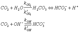
The overall rate of hydration = [CO₂] k_tot ,

where k_tot = (k_CO2 + k_OH[OH^-] ),

or the more convenient form k_tot = (k_CO2 + k_OHK_w /[H⁺]), where K_w is the dissociation constant for water, since k_OHK_w is the constant actually measured (*see note below regarding the activity of H⁺)

Both reaction rates increase with temperature. Between O^oC and 30^oC, k_CO2 increases from about 0.002 to about 0.05 s^-1 and k_OH increases from about 850 to 1400 s^-1mol^-1. Note that K_w also increases with temperature (see also table 7-1 and Section 7.3.2 ). Formulae for the kinetic and thermodynamic constants used in later calculations will be given in Section 6.2 .

Only two papers, by Miller and Berkshire (1971) and Johnson (1982), report direct measurements of these rate constants in seawater, whose high ionic strength might be expected to influence the rate, compared to more dilute solutions. There is some uncertainty, particularly regarding the rate constant k_OHK_w, which may have a significant bearing on the interpretation of the experimental results of this thesis as discussed in Section 7.7 . Therefore the measurement techniques will be introduced below.

Miller and Berkshire (1971) bubbled a stream of gas (N₂ or air) vigorously through a solution of artificial seawater, whose pCO₂ had been raised or lowered in advance to set up a disequilibrium. They used a glass electrode to measure the change in pH as a function of time. This indicates the rate of CO₂ transfer between the bubbles and solution, which is a function of both the gas exchange rate, and the reaction rate, but the former should be constant whereas the latter should increase with pH, due to the OH- reaction. By an iterative analysis of the data of dpH/dt as a function of pH, it is possible to determine the single value of the gas exchange rate which produces a straight line plot of k_tot versus [H⁺]^-1 (*see note below) as required, and from the intercept and slope of this line, to determine k_CO2 and k_OHK_w respectively. In practice a more accurate determination was found by iterating between analyses of high pH and low pH runs, in which k_OHK_w and k_CO2 dominate respectively. The rates were determined at three temperatures (constant salinity) and two salinities (constant temperature).

Miller and Berkshire (1971) noted that bubbling methods mimic the steady-state conditions of air-sea exchange fairly well, but do not work so well in freshwater, due to the larger bubbles.

Johnson (1982) bubbled 5% CO₂ in N₂ sufficiently rapidly through seawater (2400 ml min^-1 gas flow through 50ml of seawater), such that the total gas transfer rate was independent of the bubbling rate. Instead of observing a pH change over time, he kept the pH constant by titrating automatically with NaOH and recording the amount added. The total hydration and dehydration reaction rates were found by a non-linear least-squares fit to the data of bicarbonate accumulation over time. The total reaction rates were separated into k_OH and k_CO2, by repeating the experiment at a series of fixed pH values and plotting k_tot versus [H⁺]^-1 (*see note below) as above, for each combination of temperature and salinity investigated.

Both Miller and Berkshire (1971) and Johnson (1982) reported similar values of k_CO2 (within 15%). There was little salinity dependence, and the values of k_CO2 were fairly close to those previously reported for freshwater (e.g. by Pinsent et al 1956). Johnson (1982) compared his results with ten such literature values, after making a small correction for infinite dilution based on transition state theory, and found that they all agreed to within 20%.

However, the values of k_OHK_w reported by Miller and Berkshire (1971) are about 25-50% larger than those reported by Johnson (1982), the discrepancy being greater at higher temperatures. Miller and Berkshire (1971) stated that the two reaction pathways are of approximately equal importance at pH= 8.2, whereas the equivalent figure from Johnson (1982) is pH=8.45. Miller and Berkshire (1971) acknowledged that his results depended on the accuracy of literature values of K₁ and K₂ (see Section 1.2.1 ), which were uncertain at the time. Therefore a reanalysis of the experimental data using the latest equilibrium constants might be valuable.

Both workers found that k_OHK_w increased with salinity, the values in seawater being roughly double those in freshwater. This complicates comparison with other published results for freshwater, among which there is also some discrepancy, as discussed by Williams (1983), whose measurement of k_OH in alkaline lake water supports the higher values of Pinsent(1956).

*Note regarding the activity of the hydrogen ion [H⁺]

For simplicity, I have referred above to the concentration of the hydrogen ion [H⁺], rather than its activity a_H. In seawater, the activity is considerably lower than the concentration due to the high ionic strength. However, to calculate the activity of H⁺ would require the use of an activity coefficient, which cannot actually be measured in isolation from other ions, and is variable with temperature, salinity etc.. Consequently, marine chemists make use of "apparent" equilibrium constants derived from measurements in seawater at various temperatures and salinities, which incorporate the activity coefficient of H⁺ (see for example Dickson 1993, also Section 6.2 and references therein).

Reaction rates, as well as equilibria, are actually dependent on activities not concentrations. Miller and Berkshire (1971) explain that their measurements of the rate constant k_OHK_w were based on the slope of a plot of k_tot versus measured [H⁺]^-1, but since [H⁺]^-1 was derived from pH measured with an electrode, we can assume that, strictly speaking it was actually a plot of k_tot versus the activity a_H^-1. In the case of Johnson (1982), this is stated explicitly. Therefore, their reported values of k_OHK_W should be divided by the activity of the hydrogen ion, before adding to k_CO2 to get k_tot.

Since the activity is always lower than the concentration, the "apparent" rate constant should be increased when used in conjunction with the concentration of [H⁺]. However, Emerson (1995), for reasons which are not fully explained, multiplied the values of k_OHK_W from Johnson (1982) by the activity of the hydroxyl ion (taken to be 0.2), thus making the calculated OH- reaction rate much slower. I believe this adjustment of the rates is incorrect, which affects the conclusions of Emerson (1995), regarding the importance of the OH- reaction pathway. It should be noted that Boutin et al (1997), also used these corrected constants from Emerson (1995). The experimental results discussed later in Section 7.5 and Section 7.7 suggest that, if anything, the OH- reaction rate should be considerably higher than reported by Johnson (1982).

1.5.3 Algebraic reaction-diffusion models for air-sea CO₂ transfer.

The theoretical reaction-diffusion models of air sea CO₂ exchange developed by Bolin (1960), Hoover and Berkshire (1969), and Smith (1985) are all based on the stagnant film model (see Section 1.2.4 ). Differential equations describe the change in concentration of molecular CO₂ and HCO₃^-, as a function of height in the film. To solve these differential equations, some simplifying assumptions must be made. These assumptions distinguish the models, which are otherwise very similar. However, since each author used different symbols, input parameters and kinetic and thermodynamic constants, the formulae look quite different, and the reported numerical values for chemical enhancement are not comparable.

Bolin (1960) ignored the OH- reaction pathway in his calculations, because the data available at that time suggested that it was not important in typical seawater. This simplification, however, is easily remedied. Hoover and Berkshire (1969) included the OH- reaction pathway, but simplified the equations of Bolin (1960) by making use of hyperbolic identities.

The formula derived by Hoover and Berkshire is as follows:

k_en = enhanced transfer velocity (reaction+diffusion) = α k_un

k_un = diffusion-only transfer velocity

α = enhancement factor = t / [ ( t-1) + ( tanh ( b) / b) ] (note tanh =hyperbolic tangent)

t = TCO₂ / ( [HCO3-] + [CO32-] ) = 1 + ( [H⁺]² / ( K₁K₂ + K₁[H⁺] ) ) (in bulk water)

b = d * √ (k_tot t / D) (note k_tot is reaction rate, see Section 1.5.2 )

D = diffusivity of CO₂ in seawater

δ = stagnant film thickness = D / k_un (see Section 1.2.4 )

The earlier models include the diffusion of both molecular CO₂ and HCO₃^-. However, Smith (1985) made a further simplifying assumption, that the concentration of HCO₃^- is effectively constant, because it is typically at least 100 times greater than the amount of CO₂ reacting. This simplification removes the need to calculate the full speciation of the carbonic acid system, in order to calculate the chemical enhancement factor. The formula of Smith (1985) is as follows:

α = rδ / tanh (rδ), where r = √(k_tot / D)

(using the same notation as above)

This identical to the formula of Hoover and Berkshire (1969) if the ratio τ is equal to one.

1.5.4 Iterative reaction-diffusion models for air-sea CO₂ transfer

The models of Bolin (1960), Hoover and Berkshire (1969), and Smith (1985) assume that pH is constant across the stagnant film, and equal to the bulk pH (hence τ is constant). This assumption was criticised by Quinn and Otto (1971), on the grounds that if CO₂ is reacting with water, some H⁺ must be created or consumed in the microlayer, and so there will be a pH gradient. Hoover and Berkshire (1969) justified the constant pH assumption on the basis that H⁺ diffuses much faster than HCO₃^-, but Quinn and Otto (1971) pointed out, that if one species moves faster than the other, this violates the rule of electroneutrality for each sublayer of the film, and they replaced the constant pH assumption with that of electroneutrality. However, this causes the set of differential equations to become non-linear, and so they cannot be solved algebraically to produce a simple formula, and the enhancement factor must be calculated iteratively for each case. Quinn and Otto (1971) compared enhancement factors calculated this way, with those predicted by the Hoover and Berkshire formula using the same data, and found that the constant pH assumption resulted in an overprediction of the enhancement factor. Essentially, this is because the pH in the microlayer adjusts to reduce the reaction disequilibrium. How ever the overprediction was only significant for a film thickness δ>400 m m, 10 times greater than typical at sea.

Quinn and Otto (1971) also found that, when the pH was allowed to vary in the microlayer, the transfer velocity for CO₂ evasion was slightly greater than that for CO₂ invasion, for the same D pCO₂ and a constant bulk pH of 8.0. This may be explained by considering that, for CO₂ evasion, pCO₂ in the microlayer is lower, therefore the microlayer concentration of [H⁺] is slightly lower, and there is slightly less "back reaction". Note that the OH- reaction would also be greater when microlayer pH is higher, but this was not included in Quinn and Otto's model. The importance of microlayer pH is discussed further in relation to the experimental results in Section 7.5.2 .

It is important to remember that Quinn and Otto's use of "invasion" and "evasion" apply only to a situation with constant water pCO₂, and varying air pCO₂. In the calculation of the net global air-sea CO₂ flux, the variation in air pCO₂ is almost negligible, compared to that of water pCO₂. In this case, the variation in water pCO₂ will be the main influence on the microlayer pH, so the asymmetry will be different.

Even the electroneutrality assumption is not strictly true on a microscale, because some ions (particularly H⁺ and OH^-) diffuse faster than others. This creates a slight potential gradient, which alters the driving force for diffusion of other ions. To account for this, Emerson (1975a) developed a sophisticated iterative multi-layer reaction-diffusion model including all the main ionic species in seawater, each of which diffused at a different rate depending on its diffusivity and the local potential gradient, according to the formula of BenYaakov (1972). The many simultaneous equations were solved using a computer program, which alternately calculated (for a short time interval) the fluxes due to reaction in each sublayer of the stagnant film, and then the fluxes due to diffusion of each ion between sublayers, until steady-state was reached. Typically, there were about 20 sublayers, and the program looped about 1000 times (each loop representing 0.1s). Consequently, it took the computer many minutes to calculate just one enhancement factor.

Emerson (1975b) applied this computer model to calculate the chemical enhancement for a eutrophic lake, which had low salinity but high alkalinity, and a pH of about 10. In this case, at typical windspeeds the calculated enhancement factor was in the range 5-10, which agreed with an approximate estimate of the CO₂ invasion rate calculated using the biological uptake derived from the nutrient balance in the lake. The very high enhancement is due primarily to the high concentration of OH- at this high pH. In this particular case, including the effect of the potential gradient in the model made a large difference to the results. However, when the same model was applied to seawater (Emerson 1995 and personal communication), the potential gradient effect was very small, and the result was similar to that predicted by the simpler model of Quinn and Otto (1971). This is due to the high concentration of unreactive salt ions in seawater, which rapidly diffuse to counteract any potential gradient set up by reactive species. Therefore, it is reasonable to use the simpler, more convenient models to calculate enhancement factors in seawater.

Keller (1994) also developed an iterative, multilayer reaction-diffusion computer model, based instead on the "surface renewal" model of gas exchange (see Section 1.2.4 ). This did not include the effect of the potential gradient on ion diffusivities, but it did include the OH- reaction pathway. A thick "stagnant" film was divided into layers, with initial concentrations set to be the same as in the bulk water. Diffusion and reaction were alternated at short time intervals, as above, but stopped on reaching the surface renewal time, rather than allowing the system to reach steady state. This model predicted 40% higher enhancement factors, compared with an equivalent stagnant film model using the same data. This is because each time a fresh parcel of bulk water is brought to the surface, a new maximum chemical disequilibrium is set up. Moreover, HCO₃- diffuses more slowly than CO₂, and the surface renewal model is less dependent on the diffusivity than the film model (see Section 1.2.4 ). However, the iterative stagnant film model predicted lower values than the approximation of Hoover and Berkshire (1969) or Smith (1985), in agreement with the result of Quinn and Otto (1971).

Finally, we should recall that the chemical enhancement of air-water CO₂ exchange is significant, not only for calculating fluxes between the atmosphere and ocean or large lakes, but also for ecological studies of small ponds, in which there may be intense biological activity, but little turbulent mixing. Portielje and Lijklema (1995) developed an iterative multilayer reaction-diffusion model appropriate to such a system, and used it to model CO₂ fluxes into experimental ditches. Kirk and Rachhpal-Singh (1992) derived a similar model for a rice-paddy, in which both invading CO₂ and evading ammonia react with water and affect the microlayer pH, and have to be considered simultaneously.

1.5.5 Laboratory measurements of chemical enhancement

Chemical enhancement can be determined experimentally either by simultaneously measuring the transfer velocity of CO₂ and an inert gas with a similar diffusivity (such as N₂O or O₂), or by measuring the transfer velocity of CO₂ before and after acidification of the water, in otherwise identical conditions. The latter provides an effective "control", because enhancement by reaction is only significant in waters with a pH similar to or higher than that of seawater. Since seawater is corrosive, most wind-tunnel investigations of air-water gas exchange have been made using freshwater. Consequently, most experimental measurements of chemical enhancement in seawater have been in relatively small laboratory tanks.

Note that all the measured and predicted enhancement factors reported in the five papers mentioned below, are brought together later in one plot, Figure 7-14, for comparison with the new experimental results from this work as discussed in Section 7.8 . For consistency I recalculated the predictions using the formula of Hoover and Berkshire (1969) and the latest kinetic and thermodynamic constants (see Section 6.2 ), where sufficient experimental information was available.

Hoover and Berkshire (1969) made the first experimental determination of the enhancement factor in a small stirred tank, measuring evasion of ¹⁴C labelled bicarbonate from a buffered freshwater solution of pH » 6.5, with a control experiment at pH 3. The results seemed to match the predicted enhancements quite well, although Quinn and Otto (1971) suggested that surface evaporation might have influenced the transfer velocity.

Liss (1973) simultaneously measured transfer velocities of CO₂ (also with labelled ¹⁴C) and O₂ in a small stirred tank using buffered water at various pHs. The measured enhancement factor rose from one at pH 2.8, to 1.13-1.48 in buffered freshwater at pH 5.9-6.5, up to 1.62 in seawater at pH 8.2 (equivalent predictions are not given). Liss (1973) also reports similar measurements in a wind tunnel using freshwater with pH 6.2-6.6. The highest enhancement factor (at the lowest windspeed) was 1.61, 12% greater than the reported prediction.

Peng (1973, see also Broecker and Peng 1974) made simultaneous measurements of transfer velocities of CO₂, O₂ and Rn in a small stirred tank, containing either seawater or buffered freshwater at pH 8.2. The measured enhancements were much greater than those predicted, by a factor of up to 3 (see figure 7-14).

More recently, DeGrandpre et al (1995) made simultaneous measurements of CO₂ and O₂ transfer velocities in a small annular wind-wave tank, comparing distilled water (pH 5.5), spring water (pH 7.7) and seawater (pH 8.1). Results are shown as a function of mean square slope of the waves, and clearly show the importance of chemical enhancement at low windspeeds, with a maximum enhancement factor of 2.2, compared to a Hoover and Berkshire prediction of 1.35 for the same conditions (my calculation -see figure 7-14).

Finally, Wanninkhof and Knox (1996) made simultaneous measurements of CO₂ and N₂O transfer velocities, in a small stirred laboratory tank, using both seawater and acidified freshwater. Generally, there was little or no enhancement in the acidified water, but significant enhancement, up to a factor of 1.5 in the seawater at the lower stirring speeds. The measured and predicted enhancements seem to match quite well.

Wanninkhof and Knox (1996) also made some direct measurements of chemical enhancement in five lakes, using a floating helmet to trap a headspace of air whose pCO₂ could be raised or lowered by flushing with a gas, thus creating a disequilibrium. Natural fluxes of N₂O and CH₄ were used to provide the diffusion only transfer velocity for calculating chemical enhancement. Four of the lakes were alkaline, with pH from 8.6 to 9.8, and one was acidic, with pH 5.0. Generally, the observed enhancements were larger than the predicted enhancements, by a factor of up to 2, but there was not a consistent pattern.

Emerson (1975) also made some measurements of the enhancement factor in a small laboratory tank using a similar procedure to Peng (1973), but using freshwater with a pH of 10, similar to that in the eutrophic alkaline lake already mentioned above. The measured enhancement factors (3.7-6.5) were just slightly greater than those predicted using his iterative model applied to the tank water, but slightly less than predicted for the lake water, which was more buffered.

From the above results, it can be seen that the Hoover and Berkshire formula underpredicts the enhancement factor in some cases, but seems to predict it quite well in others. Possible explanations for this will be discussed later ( Section 7.7 ).

1.5.6 Effect of chemical enhancement on the net global air-sea flux

Many early investigators (Bolin 1960, Kanwisher 1963, Hoover and Berkshire 1969, Quinn and Otto 1971) asserted that, while chemical enhancement was a real and measurable effect in laboratory tanks, it would have little influence on the global air-sea flux. The logic behind this was, that the global average transfer velocity predicted by the ¹⁴C data gave a stagnant film thickness of only 35 m m, and when this is applied to models of chemical enhancement, the enhancement factor is of the order of 1%. This has remained the prevailing viewpoint (e.g. Liss 1983, Emerson 1995).

The problem with this simple calculation, is that chemical enhancement is a highly non-linear function of windspeed, temperature, and water pCO₂ (for graphs illustrating this, see the experimental results in chapter 7). Therefore, considering only average conditions can be very misleading. Moreover, if there is any intercorrelation between the kinetic factor, chemical enhancement and the thermodynamic factor, D pCO₂, its effect could be greatly magnified due to the fine balance of the net global air-sea CO₂ flux. This will be considered in much more detail in Section 3.3 and chapter 9, and therefore only a brief mention of the previous literature will be given at this stage.

Wanninkhof (1992) considered that temperature was the single most important parameter determining the flux due to chemical enhancement, and proposed a simple formula for adding chemical enhancement to his parameterisation of the transfer velocity.

For a steady windspeed, his adjusted formula became:

k = [ 2.5 (0.5246 + 1.6256x10^-2 T + 4.9946x10^-4 T² ) + 0.3u² ] ( Sc / 660)^-1/2

where T is the temperature in degrees Celsius.

Note that the constant multiplied by the square of the windspeed has been lowered to 0.3, rather than 0.31, in order that the global average transfer velocity using this formula still matches that predicted from the ¹⁴C data (see Section 1.2.12 ). The chemical enhancement is derived from the Hoover and Berkshire formula (using the constants of Johnson 1982) for a fixed k_un = 1 cm.hr^-1, and will therefore overestimate enhancement at high windspeeds, as observed by Boutin and Etcheto (1995 -see below). However, the emphasis on temperature (see also Wanninkhof and Knox 1996) did correctly identify that chemical enhancement would be greatest in equatorial regions, as demonstrated by the maps in chapter 9.

Boutin and Etcheto (1995) made the first net global CO₂ flux calculation including chemical enhancement. They used the Hoover and Berkshire formula for enhancement, together with the parameterisations of the transfer velocity of both Liss and Merlivat (1986) and Wanninkhof (1992), applied to satellite windspeed data and a map of ocean pCO₂ based on the Hamburg ocean carbon cycle model (Maier-Reimer1993). The maps clearly show that chemical enhancement is most significant in the equatorial regions where windspeed is low and temperature is high. Since pCO₂ is also high in these regions, chemical enhancement decreases the net global air-sea CO₂ flux by 5%, although it increases the global average transfer velocity by 7%, using the Liss and Merlivat parameterisation. A similar global flux calculation was made by Boutin et al (1997), which also considered the effect on the flux calculated using the ¹³C/¹²C isotope ratio (see Section 1.3.7 ). The results from this paper and that of Boutin and Etcheto (1995) will be discussed further in Section 9.6 .

We should note that both the flux calculations discussed above and the enhancement formula proposed by Wanninkhof (1992) assumed a constant seawater pH, and therefore will disregard any effect of intercorrelation between the reaction via the OH- pathway and the water pCO₂. Boutin et al (1997) justify this on the basis that varying the pH within the range found at sea made a difference of only 4% to the chemical enhancement factor. However, they used the reaction rates provided in the table of Emerson (1995), in which the rate k_OHK_w was, I believe, incorrectly divided by 5 (see Section 1.5.2 and Section 7.7). Also, a seemingly very small kinetic effect, such as the variation in OH- concentration, can have a large difference on the net global air-sea CO₂ flux if it is consistently biased towards low or high pCO₂.

This was demonstrated by the simple "thought experiment" of Keller (1994), who predicted that chemical enhancement would increase the net global air-sea CO₂ flux by about 15%, principally because the OH- reaction pathway is biased towards low pCO₂. Unfortunately, however, this calculation entirely neglected the effect of temperature variation, which increases chemical enhancement in areas of high pCO₂. Moreover Keller overestimated the effect of asymmetry in the transfer velocity, because he assumed that the ratio of the annual net global air-sea CO₂ flux, to the absolute sum of the local, short-term fluxes was only 2 : 92, whereas it is in fact considerably larger. This is due to a misinterpretation of the meaning of the "gross flux" given by the ¹⁴C data, as mentioned in Section 1.3.8 .

Nevertheless, Keller's analysis, summarised by his metaphor that the ocean can "breathe in" CO₂ a little bit faster than it can breathe it out, is a critical reminder of the importance of intercorrelation between kinetic and thermodynamic parameters. A kinetic effect, such as the OH- reaction, which seems to make little difference to the global average transfer velocity (and even less difference to the transfer velocity in average conditions), may still become significant when calculating the net global air-sea CO₂ flux. The same may apply to catalysis by the enzyme carbonic anhydrase, which will be introduced in the next chapter.

Continue to Chapter 2:
Introduction: Carbonic Anhydrase in Marine Algae and the Sea-surface Microlayer

If you jumped into this page from elsewhere, you may find it more convenient to go to the "frames" version of this thesis, alternatively you can use the links below to jump straight to a particular chapter:

Title Page Abstract Contents Figures Overview Chapter1 Chapter2 Chapter3 Chapter4 Chapter5 Chapter6 Chapter7 Chapter8 Chapter9 Chapter10 Appendix References Acknowledgements Links Download

---

Hits since 21st April 2000

---